Data tidying with tidyr

Overview

Teaching: 30 min
Exercises: 60 min

Questions

• How can I turn my dataset into the tidy format to perform efficient data analyses with R?

• How can I convert from the tidy format to a more classic wide format?

• How can I make my dataset explicit for all combinations of variables?

Objectives

• Be able to convert a dataset format using the gather and spread functions

• Be capable of understand and explore a publically available dataset (gapminder)

Table of contents

1. Introduction
2. tidyr basics
3. Explore the gapminder dataset
4. gather() data from wide to long format
5. Plot long format data
6. spread(): from long to wide format
7. Recap: the complete RMarkdown notebook
8. complete() turns implicit missing values into explicit missing values

Introduction

Now you have some experience working with tidy data and seeing the logic of wrangling when data are structured in a tidy way. But ‘real’ data often don’t start off in a tidy way, and require some reshaping to become tidy. The tidyr package is for reshaping data. You won’t use tidyr functions as much as you use dplyr functions, but it is incredibly powerful when you need it.

Why is this important? Well, if your data are formatted in a standard way, you will be able to use analysis tools that operate on that standard way. Your analyses will be streamlined and you won’t have to reinvent the wheel every time you see data in a different way.

To make a long story short:

All messy datasets are messy in their own way but all tidy datasets look alike.

Resources

These materials borrow heavily from:

• R for Data Science: Relational Data
• R for Data Science: Tidy Data
• The original paper on tidy data

Data and packages

We’ll use the package tidyr and dplyr, which are bundled within the tidyverse package.

We’ll also be using the Gapminder data we used when learning dplyr. We will also explore several datasets that come in base-R, in the datasets package.

tidyr basics

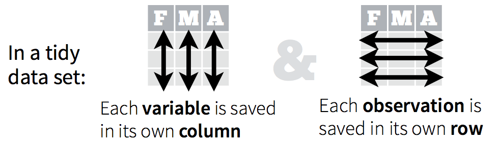
Remember, from the dplyr section, that tidy data means all rows are an observation and all columns are variables.

Let’s take a look at some examples.

Data are often entered in a wide format where each row is often a site/subject/patient and you have multiple observation variables containing the same type of data.

An example of data in a wide format is the AirPassengers dataset which provides information on monthly airline passenger numbers from 1949-1960. You’ll notice that each row is a single year and the columns are each month Jan - Dec.

In the R console, type:

AirPassengers

This format is intuitive for data entry, but less so for data analysis. If you wanted to calculate the monthly mean, where would you put it? As another row?

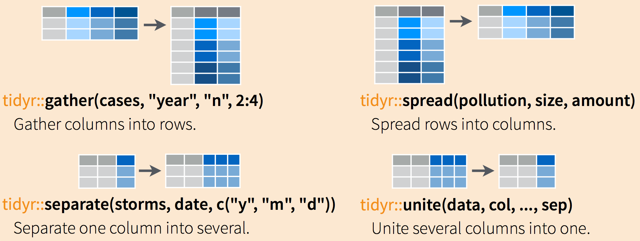
Often, data must be reshaped for it to become tidy data. What does that mean? There are four main verbs we’ll use, which are essentially pairs of opposites:

• turn columns into rows (gather()),
• turn rows into columns (spread()),
• turn a character column into multiple columns (separate()),
• turn multiple character columns into a single column (unite())

Explore the gapminder dataset.

Yesterday we started off with the gapminder data in a format that was already tidy. But what if it weren’t? Let’s look at a different version of those data.

The gapminder dataset in the wide format is on GitHub: https://raw.githubusercontent.com/ScienceParkStudyGroup/r-lesson-based-on-ohi-data-training/gh-pages/data/gapminder_wide.csv

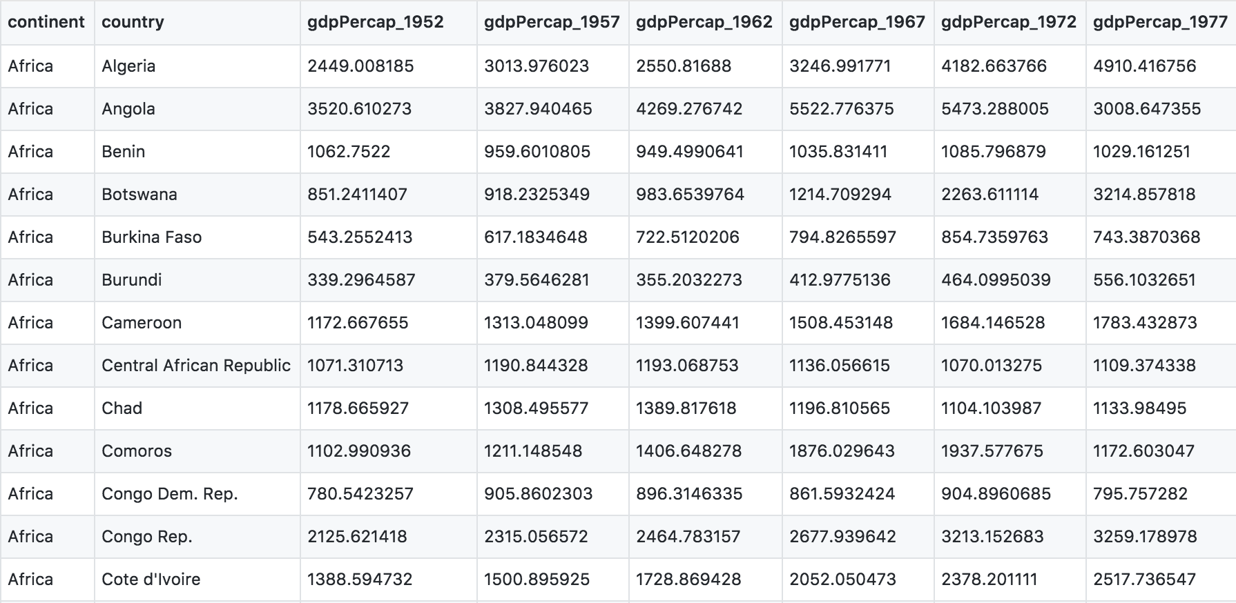
First have a look at the data.

You can see there are a lot more columns than the version we looked at before. This format is pretty common, because it can be a lot more intuitive to enter data in this way.

Sometimes, as with the gapminder dataset, we have multiple types of observed data. It is somewhere in between the purely ‘long’ and ‘wide’ data formats:

• 3 “ID variables”: continent, country, year.
• 3 “observation variables”: pop,lifeExp,gdpPercap.

It’s pretty common to have data in this format in most cases despite not having ALL observations in 1 column, since all 3 observation variables have different units. But we can play with switching it to the tidy/long* format and wide to show what that means (i.e. long would be 4 ID variables and 1 observation variable).

But we want it to be in a tidy way so that we can work with it more easily. So here we go.

You use spread() and gather() to transform or reshape data between wide to long formats.

Setup

OK let’s get going.

We’ll learn tidyr in an RMarkdown file within a GitHub repository so we can practice what we’ve learned so far. You can either continue from the same RMarkdown, or begin a new one.

Here’s what to do:

1. Clear your workspace (Session > Restart R)
2. New File > R Markdown…, save it under the gapminder-wrangle.Rmd name.

I’m going to write this outside of a coding chunk in my RMarkdown file:

Data wrangling with `tidyr`, which is part of the tidyverse. We are going to tidy some data!

Load tidyverse (which has tidyr inside)

First load tidyr in an R chunk. You already have installed the tidyverse, so you should be able to just load it like this (using the comment so you can run install.packages("tidyverse") easily if need be):

library(tidyverse) # install.packages("tidyverse")

gather() data from wide to long format

Data import

Read in the data from GitHub. Let’s also read in the gapminder data (tidy format) so that we can use it to compare later on.

## wide messy format
gap_wide <- readr::read_csv('https://raw.githubusercontent.com/ScienceParkStudyGroup/r-lesson-based-on-ohi-data-training/gh-pages/data/gapminder_wide.csv')

## long tidy format
gapminder <- readr::read_csv('https://raw.githubusercontent.com/ScienceParkStudyGroup/r-lesson-based-on-ohi-data-training/gh-pages/data/gapminder.csv')

Let’s have a look:

head(gap_wide)
str(gap_wide)

While wide format is nice for data entry, it’s not nice for calculations. Some of the columns are a mix of variable (e.g. “gdpPercap”) and data (“1952”). What if you were asked for the mean population after 1990 in Algeria? Possible, but ugly. But we know it doesn’t need to be so ugly. Let’s tidy it back to the format we’ve been using.

Discussion point

Question: let’s talk this through together. If we’re trying to turn the gap_wide format into gapminder format, what structure does it have that we like? And what do we want to change?

Solution

• We like the continent and country columns. We won’t want to change those.
• We want 1 column identifying the variable name (tidyr calls this a ‘key’), and 1 column for the data (tidyr calls this the ‘value’).
• We actually want 3 different columns for variable: gdpPercap, lifeExp, and pop.
• We would like year as a separate column.

Let’s get it to long format. We’ll have to do this in 2 steps. The first step is to take all of those column names (e.g. lifeExp_1970) and make them a variable in a new column, and transfer the values into another column. Let’s learn by doing:

Let’s have a look at gather()’s help:

?gather

Discussion point

Question: What is our key-value pair?

We need to name two new variables in the key-value pair, one for the key, one for the value. It can be hard to wrap your mind around this, so let’s give it a try. Let’s name them obstype_year and obs_values.

Here’s the start of what we’ll do:

gap_long <- gap_wide %>% 
  gather(key   = obstype_year,
         value = obs_values)

Although we were already planning to inspect our work, let’s definitely do it now:

str(gap_long)
head(gap_long)
tail(gap_long)

We have reshaped our dataframe but this new format isn’t really what we wanted.

What went wrong? Notice that it didn’t know that we wanted to keep continent and country untouched; we need to give it more information about which columns we want reshaped. We can do this in several ways.

One way is to identify the columns is by name. Listing them explicitly can be a good approach if there are just a few. But in our case we have 30 columns. I’m not going to list them out here since there is way too much potential for error if I tried to list gdpPercap_1952, gdpPercap_1957, gdpPercap_1962 and so on. But we could use some of dplyr’s awesome helper functions — because we expect that there is a better way to do this!

gap_long <- gap_wide %>% 
  gather(key   = obstype_year,
         value = obs_values,
         dplyr::starts_with('pop'),
         dplyr::starts_with('lifeExp'),
         dplyr::starts_with('gdpPercap'))  #here i'm listing all the columns to use in gather

str(gap_long)
head(gap_long)
tail(gap_long)

Success! And there is another way that is nice to use if your columns don’t follow such a structured pattern: you can exclude the columns you don’t want. This is actually what I’d recommend in most cases (less error-prone and simpler to understand).

gap_long <- gap_wide %>% 
  gather(key   = obstype_year,
         value = obs_values,
         -continent, -country)

str(gap_long)
head(gap_long)
tail(gap_long)

Recap:

Inside gather(), we first name the new column for the new ID variable (obstype_year) and the name for the new amalgamated observation variable (obs_value), then the names of the old observation variable. We could have typed out all the observation variables, but as in the select() function (see dplyr lesson), we can use the starts_with() argument to select all variables that starts with the desired character string. Gather also allows the alternative syntax of using the - symbol to identify which variables are not to be gathered (i.e. ID variables).

From messy to tidy: final steps

OK, but we’re not done yet. obstype_year actually contains two pieces of information, the observation type (pop,lifeExp, or gdpPercap) and the year. We can use the separate() function to split the character strings into multiple variables.

?separate –> the main arguments are separate(data, col, into, sep ...). So we need to specify which column we want separated, name the new columns that we want to create, and specify what we want it to separate by. Since the obstype_year variable has observation types and years separated by a _, we’ll use that.

gap_long <- gap_wide %>% 
  gather(key   = obstype_year,
         value = obs_values,
         -continent, -country) %>%
  separate(obstype_year,
           into = c('obs_type','year'),
           sep = "_",
           convert = TRUE) #this ensures that the year column is an integer rather than a character

No warning messages…still we inspect:

str(gap_long)
head(gap_long)
tail(gap_long)

Excellent. This is long format: every row is a unique observation. Yay!

Plot long format data

The long format is the preferred format for plotting with ggplot2. Let’s look at an example by plotting just Canada’s life expectancy.

canada_df <- gap_long %>%
  filter(obs_type == "lifeExp",
         country == "Canada")

ggplot(canada_df, aes(x = year, y = obs_values)) +
  geom_line()

We can also look at all countries in the Americas:

life_df <- gap_long %>%
  filter(obs_type == "lifeExp",
         continent == "Americas")

ggplot(life_df, aes(x = year, y = obs_values, color = country)) +
  geom_line()

Your turn

Exercise

1. Using gap_long, calculate and plot the the mean life expectancy for each continent over time from 1982 to 2007. Give your plot a title and assign x and y labels.
   Hint: do this in two steps. First, do the logic and calculations using dplyr::group_by() and dplyr::summarize(). Second, plot using ggplot().

Solution

Calculation
continents <- gap_long %>%
filter(obs_type == "lifeExp",
year > 1980) %>%
group_by(continent, year) %>%
summarize(mean_le = mean(obs_values)) %>%
ungroup()
Plot
ggplot(data = continents, aes(x = year, y = mean_le, color = continent)) +
geom_line() +
labs(title = "Mean life expectancy", x = "Year", y = "Age (years)")

Additional customization

We can use the scale_fill_brewer from the ggplot2 package to change the colour scheme of our plot.
From the help page of the function:

The brewer scales provides sequential, diverging and qualitative colour schemes from ColorBrewer. These are particularly well suited to display discrete values on a map. See http://colorbrewer2.org for more information.

ggplot(data = continents, aes(x = year, y = mean_le, color = continent)) + 
  geom_line() +
  labs(title = "Mean life expectancy",
       x = "Year",
       y = "Age (years)",
       color = "Continent") +
  theme_classic() +
  scale_fill_brewer(palette = "Blues")  

spread(): from long to wide format

The function spread() is used to transform data from long to wide format.

Alright! Now just to double-check our work, let’s use the opposite of gather() to spread our observation variables back to the original format with the aptly named spread(). You pass spread() the key and value pair, which is now obs_type and obs_values.

gap_normal <- gap_long %>% 
  spread(obs_type, obs_values)

No warning messages is good…but still let’s check:

dim(gap_normal)
dim(gapminder)
names(gap_normal)
names(gapminder)

Now we’ve got a dataframe gap_normal with the same dimensions as the original gapminder.

Your turn

Exercise

Convert gap_long all the way back to gap_wide.
Hint: Do this in 2 steps. First, create appropriate labels for all our new variables (variable_year combinations) with the opposite of separate: tidyr::unite(). Second, spread() that variable_year column into wider format.

Solution

head(gap_long) # remember the columns
gap_wide_new <- gap_long %>%
First unite obs_type and year into a new column called var_names. Separate by _
unite(col = var_names, obs_type, year, sep = "_") %>%
Then spread var_names out by key-value pair.
spread(key = var_names, value = obs_values)
str(gap_wide_new)

Recap: the complete RMarkdown notebook

Spend some time cleaning up and saving gapminder-wrangle.Rmd Restart R. In RStudio, use Session > Restart R. Otherwise, quit R with q() and re-launch it.

This session RMarkdown notebook .Rmd could look something like this:

## load tidyr (in tidyverse)
library(tidyverse) # install.packages("tidyverse")

## load wide data
gap_wide <- readr::read_csv('https://raw.githubusercontent.com/ScienceParkStudyGroup/r-lesson-based-on-ohi-data-training/gh-pages/data/gapminder_wide.csv')

head(gap_wide)
str(gap_wide)

## practice tidyr::gather() wide to long
gap_long <- gap_wide %>% 
  gather(key   = obstype_year,
         value = obs_values,
         -continent, -country) 
# or 
gap_long <- gap_wide %>% 
  gather(key   = obstype_year,
         value = obs_values,
         dplyr::starts_with('pop'),
         dplyr::starts_with('lifeExp'),
         dplyr::starts_with('gdpPercap'))

## gather() and separate() to create our original gapminder
gap_long <- gap_wide %>% 
  gather(key   = obstype_year,
         value = obs_values,
         -continent, -country) %>%
  separate(obstype_year,
           into = c('obs_type','year'),
           sep="_")

## practice: can still do calculations in long format
gap_long %>% 
  group_by(continent, obs_type) %>%
  summarize(means = mean(obs_values))

## spread() from normal to wide
gap_normal <- gap_long %>% 
  spread(obs_type, obs_values) %>%
  select(country, continent, year, lifeExp, pop, gdpPercap)

## check that all.equal()
all.equal(gap_normal,gapminder)

## unite() and spread(): convert gap_long to gap_wide
head(gap_long) # remember the columns

gap_wide_new <- gap_long %>% 
  # first unite obs_type and year into a new column called var_names. Separate by _
  unite(col = var_names, obs_type, year, sep = "_") %>% 
  # then spread var_names out by key-value pair.
  spread(key = var_names, value = obs_values)
str(gap_wide_new)

complete() turns implicit missing values into explicit missing values.

One of the coolest functions in tidyr is the function complete(). Jarrett Byrnes has written up a great blog piece showcasing the utility of this function so I’m going to use that example here.

We’ll start with an example dataframe where the data recorder enters the Abundance of two species of kelp, Saccharina and Agarum in the years 1999, 2000 and 2004.

kelpdf <- data.frame(
  Year = c(1999, 2000, 2004, 1999, 2004),
  Taxon = c("Saccharina", "Saccharina", "Saccharina", "Agarum", "Agarum"),
  Abundance = c(4,5,2,1,8)
)

kelpdf

Jarrett points out that Agarum is not listed for the year 2000. Does this mean it wasn’t observed (Abundance = 0) or that it wasn’t recorded (Abundance = NA)? Only the person who recorded the data knows, but let’s assume that the this means the Abundance was 0 for that year.

We can use the complete() function to make our dataset more complete.

kelpdf %>% 
  complete(Year, Taxon)

This gives us an NA for Agarum in 2000, but we want it to be a 0 instead. We can use the fill argument to assign the fill value.

kelpdf %>% complete(Year, Taxon, fill = list(Abundance = 0))

Now we have what we want. Let’s assume that all years between 1999 and 2004 that aren’t listed should actually be assigned a value of 0. We can use the full_seq() function from tidyr to fill out our dataset with all years 1999-2004 and assign Abundance values of 0 to those years & species for which there was no observation.

kelpdf %>% complete(Year = full_seq(Year, period = 1),
                   Taxon,
                   fill = list(Abundance = 0))

Other links

• Tidying up Data - Env Info - Rmd
• Data wrangling with dplyr and tidyr - Tyler Clavelle & Dan Ovando - Rmd

Key Points

• The gather function turns columns into rows (make a dataset tidy).

• The spread function turns rows into columns (make a dataset wide).

• Tidy dataset go hand in hand with ggplot2 plotting.

• The complete function fills in implicitely missing observations (balance the number of observations).