Data exploration and properties

Overview

Teaching: 60 min
Exercises: 30 min

Questions

Which packages do I need for the analyses?

How can I import my data in R?

What do the data sets look like?

What are the properties for the occurrence table?

Objectives

Install and load the required packages in R

Import the data sets

Create a phyloseq object

Explore the data sets

Assess sparsity of the occurrence table

Assess sequencing depth

1. Install and load the required packages
2. Import the data in R
3. Create a phyloseq object
4. Global exploration of the data sets
5. OTU data properties

1. Install and load the required packages

# install the following packages only if you need to
# install.packages("vegan")  
# install.packages("tidyverse")
# install.packages("patchwork")
# install.packages("agricolae")
# install.packages("FSA")
# install.packages("rcompanion")
# BiocManager::install('phyloseq') # this package comes from Bioconductor  

library(vegan)
library(phyloseq)
library(tidyverse)
library(patchwork)
library(agricolae)
library(FSA)
library(rcompanion)

2. Import the data interpretation R

data_otu <- read.table("data_loue_16S_nonnorm.txt", header = TRUE)
data_grp <- read.table("data_loue_16S_nonnorm_grp.txt", header=TRUE, stringsAsFactors = TRUE)
data_taxo <- read.table("data_loue_16S_nonnorm_taxo.txt", header = TRUE)

The OTU table (data_otu or data_loue_16S_nonnorm.txt) is the occurrence table that contains counts corresponding to the number of times each OTU (Operational Taxonomic Unit, here bacteria) is observed in each sample.

The sample metadata table (data_grp or data_loue_16S_nonnorm_grp.txt) represents the metadata information on the different samples, in this case, where (site) and when (month) the samples were harvested.

The taxonomy table (data_taxo or data_loue_16S_nonnorm_taxo.txt) represents the assignment for the different OTU at domain, phylum, class, order, family, genus and species levels. Usually, microbial ecologists use phylum level (or class level for Proteobacteria) to describe the global bacterial communities. Then, they usually use OTU, ASV (Amplicon Sequence Variant) or genus level to check which bacteria are differentially occuring in the different treatments.

3. Create a phyloseq object

Microbial ecologists usually use the vegan and phyloseq packages to analyse the occurrence table. Such as biom format, phyloseq format support encapsulation of core study data (occurrence table data and sample/observation metadata) in a single file. From the three tables data_otu, data_grp and data_taxo we will create a phyloseq object data_phylo.

OTU = otu_table(as.matrix(data_otu), taxa_are_rows = FALSE) # create the occurrence table object in phyloseq format
SAM = sample_data(data_grp, errorIfNULL = TRUE) # create the sample metadata object in phyloseq format
TAX = tax_table(as.matrix(data_taxo)) # create the observation metadata object (OTU taxonomy) in phyloseq format
data_phylo <- phyloseq(OTU, TAX, SAM) # create the phyloseq object including occurrence table data and sample/observation metadata
data_phylo # print information about the phyloseq object

This is what you should see:

phyloseq-class experiment-level object
otu_table()   OTU Table:         [ 5248 taxa and 18 samples ]
sample_data() Sample Data:       [ 18 samples by 3 sample variables ]
tax_table()   Taxonomy Table:    [ 5248 taxa by 8 taxonomic ranks ]

4. Global exploration of the data sets

4.1. OTU table

Based on raw data: data_otu table or OTU from data_phylo object. The OTU table is the occurrence table that contains counts.

Check how the data look like showing the first 5 rows and the first 6 columns.

data_otu[1:5, 1:6] # as we have here a high number of variables it is better to not use head function for a better readability

            OTU_00009 OTU_00010 OTU_00020 OTU_00025 OTU_00032 OTU_00035
Cleron_07_1         0         0         0         1         0         0
Cleron_07_2         0         0         0         0         0         0
Cleron_07_3         2         0         0         2         0         0
Cleron_08_1         1         0         0         4         0         0
Cleron_08_2         0         0         0         1         0         0

The OTU table has samples in rows and variables (OTU) in columns.

Remark

If you want to use phyloseq, you can do the same running otu_table(data_phylo)[1:5, 1:6]

Let’s check how many samples and variables there are in the OTU table.

nb_samples <- dim(data_otu)[1] # nb of rows, here samples
nb_samples

nb_var <- dim(data_otu)[2] # number of columns, here variables (OTU)
nb_var

There are 18 samples and 5248 variables.

Remark

If you want to use phyloseq, you can use nsamples() and ntaxa() functions, such as nsamples(data_phylo) and ntaxa(data_phylo).

Now, let’s check how many total sequences/reads there are in the OTU table.

sum(data_otu)

[1] 245239

In total, there are 245239 sequences/reads.

4.2. Sample metadata table

Based on data_grp table or SAM from data_phylo object. This table represents the metadata information on the different samples.

Exercise

How does the data look like if you show the first 6 rows using head function?

Solution

head(data_grp) # The sample metadata table has samples in rows and factors in columns.

Remark

If you want to use phyloseq, you can do the same running head(sample_data(data_phylo)).

Exercise

How many samples and factors are in the metadata table?

Solution

dim(data_grp)[1] # number of samples.
nb_factors <- dim(data_grp)[2] # number of factors
nb_factors

Check how many samples per treatment do we have.

summary(data_grp)

 site       month         site_month
 Cleron:9   August   :6   Cleron_August   :3   
 Parcey:9   July     :6   Cleron_July     :3   
            September:6   Cleron_September:3   
                          Parcey_August   :3   
                          Parcey_July     :3   
                          Parcey_September:3   

There are nine samples harvested or replicates (ignoring the month of harvest) for each of the two sites: Cleron (located at the upstream area of the river) and Parcey (located at the downstream area of the river). There are six replicates per month (ignoring the site of harvest). There are three replicates considering both site and month of harvest.

Remark

If you want to use phyloseq, you can do the same running dim(sample_data(data_phylo))[1], dim(sample_data(data_phylo))[2] and summary(sample_data(data_phylo)$site)

Discussion point

This is a multivariate data set with an underlying experimental design. What would be your first idea to analyze this data?

In the following part of this tutorial, we will discuss some problematic issues of these data that makes it necessary to use a specific strategy to deal with these data.

5. OTU data properties

Based on the raw data: data_otu table. Microbiome data sets are usually sparse and have an uneven library size.

5.1. Sparsity

5.1.1. Number of zeros and percentage of zeros in the OTU table

sum(data_otu == 0)
sum(data_otu == 0) / (nb_var * nb_samples) * 100

There are 68633 zeros in the OTU table which represent around 73% of the values.

Question

According to your knowledge, what could be the meaning of a zero value in the OTU/ASV table?

Can we consider it as a true zero?

Do you think that it is important to filter the data and why?

Solution

A zero value in the OTU table means that we could not sequence any read for a specific OTU/ASV in a given sample. This means that there is not such OTU/ASV in the given sample or that the sequencing depth was not enough to find it.

So, we usually don’t know if it is a true zero or not.

First, some statistical approcahes cannot handle highly sparse data set (for example Principal Component Analysis).
Then, there is often problem when we have to compare rare OTU/ASV. For example, if for one sample you cannot find any count for a specific OTU but for another sample you can find 1 count for this OTU, can you say that there is more of this OTU in the second sample than in the first one?
Therefore, in the context of microbiota data analysis, zeros values can be difficult to analyse and interpret and data should often be filtered.

Remark

Here, the percentage of zeros is relatively high. In order to be able to apply specific statistical approaches later, we should think about filtering the OTU data.

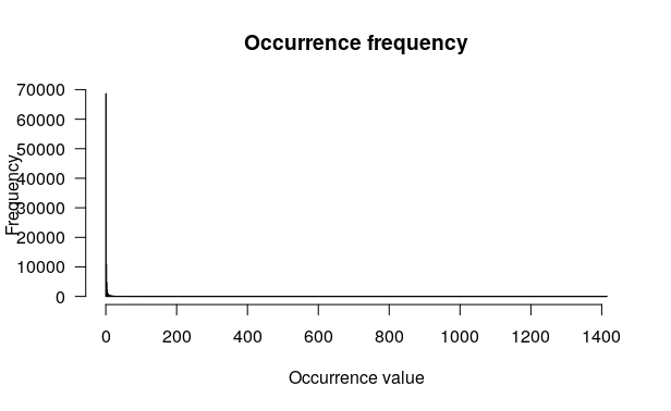
5.1.2. Counts frequency

Visualize the count frequency in the OTU table using a histogram.

hist(as.matrix(data_otu), 
     max(data_otu), 
     right = FALSE, 
     las = 1, 
     xlab = "Occurrence value", 
     ylab = "Frequency", 
     main = "Occurrence frequency")

Question

How do you interpret this histogram?

Solution

This plot represents the occurence frequency. The x axis represents the occurence value (for the all OTU table, so for each sample and OTU) and y the frequency.
You can see that for x = 0, y = 68633. So, there are 68633 zeros in the OTU table.
You can also see that the histogram is rapidly decreasing as x increases. This means that there is a lot of low counts > > occurences (such as 0, 1 or 2 counts per OTU and per sample) and few abundant OTU.

Remark

One option for data fitering could be to remove OTUs that have a total count over all samples per OTU lower than a defined value.

5.1.3. Minimum total count over all samples per OTU

Question

What is the minimum total count over all samples per OTU in this data set?

Solution

min(colSums(data_otu))

Remark

As illustrated in this tutorial, after the first bioinformatic analysis that generate the OTU table, microbial ecologists usually remove singletons (OTU for which only one read has been identified in the full OTU table, including all the samples).
Microbial ecologists consider that reads which are present only once should be treated as artifacts and removed. As a reminder, chimeric amplification products have been already removed in the bioinformatic analysis before generating the OTU table. Chimeras are hybrid products between multiple parent sequences that can be falsely interpreted as novel organisms, thus inflating apparent diversity.
thus inflating apparent diversity.

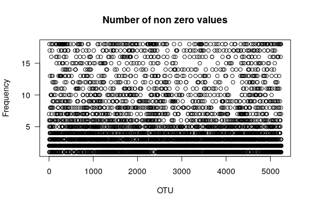
5.1.4. Non-zero values per OTU

In order to check how the different OTU/ASV are shared bewteen samples, plot the number of non-zero values for each OTU

non_zero <- 0*1:nb_var

for (i in 1:nb_var){
  non_zero[i]<-sum(data_otu[,i] != 0)
  }

plot(non_zero, xlab = "OTU", ylab = "Frequency", main = "Number of non zero values", las = 1)

Question

How do you interpret this plot?

Solution:

This plot represents the number of non-zero values. The x axis represents the different OTU (we have here 5248 OTU) and the y axis represents the frequency (from 1 to 18, as we have 18 samples).
You can see that there is a lot of dots when y < 5, which means that the major part of the non-zeros values are found in less than 5 samples. We can also say that there are few non-zero counts that are shared in more than 5 samples.
The major part of the OTU are thus specific to only a few number of samples.

Remark

Remember that, here, the number of replicates per treatment is 3 per site and per harvesting date, 6 per harvesting date, and 9 per site.
We can think about different ways to filter the OTU data. For example, here, we can think about removing rare OTU that are not shared with at least 2 or 3 samples. Try to think about how you can filter your OTU data.

5.2. Sequencing depth

Sequencing depth and library size represent the number of counts per sample. This number can vary a lot among the different samples, usually up to 10 fold between some samples and it is especially due to several technical biases. Some of these biases are explained below.
After extracting the DNA from each sample independently, the biologist measures the DNA concentration for each sample. First, the sensitivity of the technique used to measure DNA concentration is not always very high. Then, according to this concentration, the biologist pools the different samples in one equimolar mix using pipette, which add also some error. Moreover, the PCR amplification step can also add some difference among samples because PCR amplification can be more/less efficient according to the sequence itself.

Question

Why do you think that it is important to look for sequencing depth?

Solution:

First, it is important to know if we sequenced enough to catch all the diversity present in our environment.
Then, if you want to be able to compare the samples to each others, we need to have a comparable library size between samples.

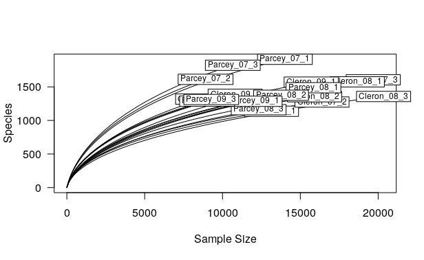
5.2.1. Rarefaction curve

Microbial ecologists explore sequencing depth though a rarefaction curve. The rarefaction curve shows how many new OTU are observed when we obtain new reads for a given sample. If the sequencing depth is enough, we should observe a plateau, meaning that even if we sequence new reads they will belong to OTUs already observed. In other word, all the diversity present in a sample is already described and we have sequenced the community deeply enough. This analysis should be execute on the raw data.

Remark

We check sequencing depth on the raw data: data_otu.

The parameter step is used here to decrease computation time. step = 100 means that the rarefaction curve will be calculated and plotted only for sample size = 1, 101, 201, (…), and maximun value.

rarecurve(data_otu, step = 100, cex = 0.75, las = 1) 

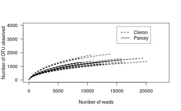
We can also customize the plot: adding title, legend, etc.

par(cex = 1, las = 1)
leg.txt <- c("Cleron", "Parcey")
lty_vector <- c(2,2,2,2,2,2,2,2,2,2,2,2,1,1,1,1,1,1,1,1,1,1,1,1)
rarecurve(data_otu, 
	step = 100, 
	lwd=1.3, 
	xlab = "Number of reads", 
	ylab = "Number of OTU observed", 
	xlim = c(-50, 23000), 
	ylim = c(-5, 4000), 
	label = FALSE, 
	lty = lty_vector) 
legend(15000, 3900, leg.txt, lty = c(2,1), lwd = 1.3, box.lwd = 0.6, cex = 1)

Question

How do you interpret this plot? Do you think that the sequencing depth was enough for this experiment?

Do you think it is possible to compare the samples using this data set?

Solution:

You can see that none of the samples reach a plateau, so the sequencing depth was not enough, but we should not be so far from it. Our previous comparison between Richness and Chao1 give us the same interpretation.

You can also see with this plot that the total number of reads per sample vary between samples, so it will be difficult to compare samples.

5.2.2. Library size

We will now plot the total number of counts per sample.

sum_seq <- rowSums(data_otu)
plot(sum_seq, ylim=c(0,25000), main=c("Number of counts per sample"), xlab=c("Samples"))
sum_seq

Cleron_07_1 Cleron_07_2 Cleron_07_3 Cleron_08_1 Cleron_08_2 Cleron_08_3 Cleron_09_1 
      13146       16390       19685       18657       15916       20347       15698 
Cleron_09_2 Cleron_09_3 Parcey_07_1 Parcey_07_2 Parcey_07_3 Parcey_08_1 Parcey_08_2 
       8726       10814       14009        8914       10661       15842       13760 
Parcey_08_3 Parcey_09_1 Parcey_09_2 Parcey_09_3 
      12323       12066        9008        9277 

min(sum_seq)
max(sum_seq)

[1] 8726
[1] 20347

Questions

How do you interpret these results?

Do you think it is an issue to have variation in the library size?

Solutions:

We can see that there is differences in the library size for the different samples. The library size go from around 9000 reads to a bit more of 20000 reads (more than 2 fold change).

Of course if you want to compare samples to each other, it will be an issue to have different library sizes. For example, if you have a sample 1 with 1000 reads (500 reads for OTU1, 300 reads for OTU 2 and 200 reads for OTU 3) and a sample 2 with only 100 reads (50 reads for OTU1, 30 reads for OTU 2 and 20 reads for OTU 3). If you are comparing the two samples without correcting for the library size, you will say that sample 2 as 10 times less OTU 1, 2 and 3 than the sample 1, while it is just due to the difference in library size. Indeed, if you calculate the percentage, you will have 50% of OTU 1, 30% of OTU 2 and 20% of OTU 3 for both samples. So, > > it is important to normalize your data per sample.

Remark

We observe here a diffrence of around 2.3 fold change between the lowest and the highest library size. However, usually differences among samples are bigger (up to 10 fold). This is probably due to the fact that we have only a subset of the data here (not all the treatments were kept).

Key Points

previous episode

Microbiota data analysis

next episode

Data exploration and properties

Overview

Table of Contents

1. Install and load the required packages

2. Import the data interpretation R

3. Create a phyloseq object

4. Global exploration of the data sets

4.1. OTU table

Remark

Remark

4.2. Sample metadata table

Exercise

Solution

Remark

Exercise

Solution

Remark

Discussion point

5. OTU data properties

5.1. Sparsity

5.1.1. Number of zeros and percentage of zeros in the OTU table

Question

Solution

Remark

5.1.2. Counts frequency

Question

Solution

Remark

5.1.3. Minimum total count over all samples per OTU

Question

Solution

Remark

5.1.4. Non-zero values per OTU

Question

Solution:

Remark

5.2. Sequencing depth

Question

Solution:

5.2.1. Rarefaction curve

Remark

Question

Solution:

5.2.2. Library size

Questions

Solutions:

Remark

Key Points

previous episode

next episode