Finding tissue-specific genes through feature engineering
Overview
Teaching: 0 min
Exercises: 45 minQuestions
How do I transform my variables to build more meaningful variables?
What type of transformation and checks should I perform?
How to extract my list of selected tissue-specific genes?
Objectives
Understand how distances are calculated between two tissues based on their gene expression profile.
Be able to name a few different clustering methods.
Table of Contents
1. Introduction
There is an alternative perhaps more intuitive method to find tissue-specific genes. Actually this is the method used by Ahn and co-authors in their publication.
Here are the different steps that will be undertaken:
- Create a dataframe that only contains the gene TPM values for our tissue of interest (e.g. subcutaneous adipose tissue)
- Create a dataframe that contains all other tissues gene TPM values.
- Compute the median TPM value per gene for the other tissues.
- Join the two dataframes.
- Calculate the subcutaneous adipose versus _all other tissues__ fold changes.
- Converting this fold change to a \(log_{2}\) fold change to normalise the distribution of the fold changes.
- Perform a \(Z\)-test analysis to compute p-values.
- Extract the genes with the highest and most significant \(log_{2}\) fold changes.
2. Feature engineering
Here, feature engineering refers to the grouping of the other tissues under a new variable called “other_tissues”. This will turn our complex multivariate analysis (see PCA and clustering episodes) into a simpler univariate analysis.
2.1 Filtering genes with low expression values
Import or re-import the data first.
df_expr <- read.delim(file = "data/GTEx_Analysis_2016-01-15_v7_RNASeQCv1.1.8_gene_median_tpm.tsv",
                      header = TRUE,
                      stringsAsFactors = FALSE,
                      check.names = FALSE)


df_expr_tidy <- df_expr %>%
  select(- Description) %>%
  pivot_longer(- gene_id, names_to = "tissue", values_to = "tpm")
threshold = df_expr_tidy %>%
  group_by(gene_id) %>%
  summarise(median_tpm = median(tpm)) %>%
  with(., round(x = quantile(x = median_tpm, probs = 0.9)))

genes_selected =
  df_expr_tidy %>%
  group_by(gene_id) %>%
  summarise(median_tpm = median(tpm)) %>%
  ungroup() %>%
  filter(median_tpm > threshold) %>%
  dplyr::pull(gene_id)

df_expr_tidy_filtered <- filter(df_expr_tidy, gene_id %in% genes_selected)
2.2 Creating the adipose and other tissues dataframes
# extract gene TPM value in "Adipose - Subcutaneous"
adipose_gene_expression <- df_expr_tidy_filtered %>%
  filter(tissue == "Adipose - Subcutaneous") %>%
  select(gene_id, tpm) %>%
  rename(adipose_tpm = tpm)

# calculate median TPM value in all other tissues
all_other_tissues_gene_expression <-
  df_expr_tidy_filtered %>%
  filter(tissue != "Adipose - Subcutaneous") %>%
  group_by(gene_id) %>%
  summarise(other_tissues_median_tpm = median(tpm))
2.3 Merge dataframes and calculate log2 fold changes
## Merge the two dataframes
## Calculate a fold change
adipose_vs_other_tissues <- inner_join(x = adipose_gene_expression,
                                       y = all_other_tissues_gene_expression,
                                       by = "gene_id") %>%
  mutate(fc = adipose_tpm / other_tissues_median_tpm) %>%
  mutate(log2_fc = log2(fc))
3. Compute \(Z\)-tests and extract adipose-specific genes
Since our sample size is relatively large (> 50), we can perform a \(Z\)-test analysis to compute the probability
3.1 Normality test
# normal distribution of log2FC?
ggplot(adipose_vs_other_tissues, aes(x = log2_fc)) +
  geom_density()

  # calculate Z-score
mean_of_log2fc <- with(data = adipose_vs_other_tissues, mean(log2_fc))
sd_of_log2fc <- with(data = adipose_vs_other_tissues, sd(log2_fc))

# test for normality
ks.test(x = adipose_vs_other_tissues$log2_fc, y = "pnorm", mean = mean_of_log2fc, sd = sd_of_log2fc)
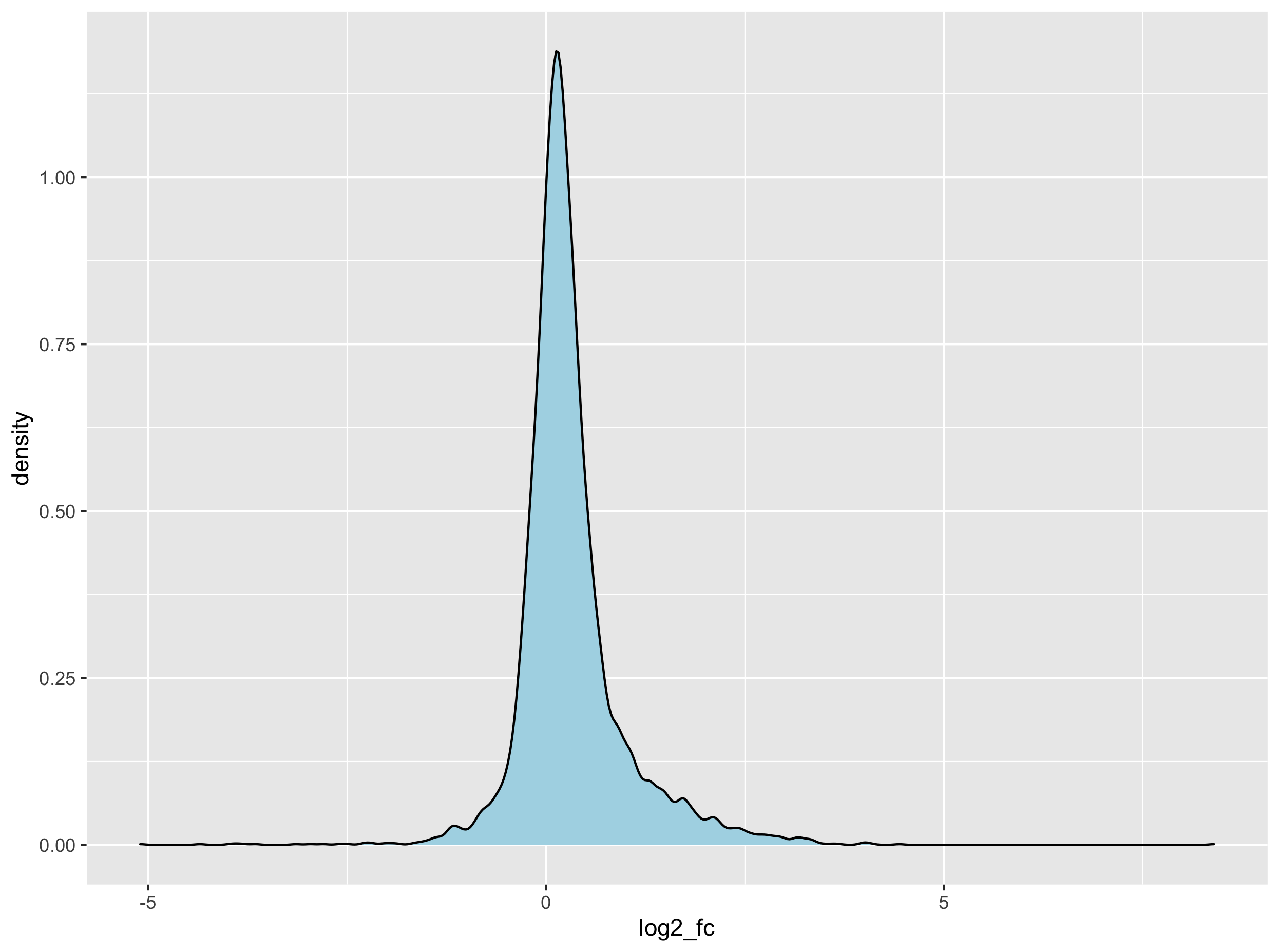
The Kolmogorov–Smirnov test that compares the observed distribution of the \(log_{2}\) fold change to its theoretical normal distribution (based on its observed mean and variance). The null hypothesis stipulates that the observed distribution are drawn from its theoretical normal distribution. A large \(D\) score will convert to a small p-value therefore suggesting that the distribution significantly deviates from its theoretical normal distribution.
One-sample Kolmogorov-Smirnov test

data:  adipose_vs_other_tissues$log2_fc
D = 0.14537, p-value < 2.2e-16
alternative hypothesis: two-sided
Although our data is not strictly normal sensu stricto, we will assume it is for demonstration purposes and since a high \(log_{2}\) will nethertheless indicate a high expression in subcutaneous adipose tissue.
3.2 \(Z\)-test
The \(Z\)-test can be used to test whether an observed \(log_{2}\) fold change is significantly different from the population average \(log_{2}\) fold changes. To perform this analysis, we can compute the \(Z\)-score for each of the \(log_{2}\). In turn, this allows to convert this score to a probability for each of the individual gene fold change.
adipose_vs_other_tissues$zscore <- map_dbl(
  adipose_vs_other_tissues$log2_fc,
  function(x) (x - mean_of_log2fc) / sd_of_log2fc
  )
3.3 Compute p-values and extract final list
Here, p-values will be extracted using a one-tailed p-value since we want log2 fold changes higher than
# filter fc > 0 + calculate one-sided p-value
adipose_specific_genes =
  adipose_vs_other_tissues %>%
  filter(log2_fc > 0) %>%                   # FC superior to 1
  mutate(pval = 1 - pnorm(zscore)) %>%      # one-tailed p-value
  filter(pval < 0.01) %>%
  arrange(desc(log2_fc))

head(adipose_specific_genes, n = 10)
This yields the top 10 genes:
# A tibble: 10 x 7
   gene_id           adipose_tpm other_tissues_median_tpm    fc log2_fc zscore     pval
   <chr>                   <dbl>                    <dbl> <dbl>   <dbl>  <dbl>    <dbl>
 1 ENSG00000170323.4       5946.                     17.7 336.     8.39  12.1  0.
 2 ENSG00000196616.8       1302                      60.0  21.7    4.44   6.16 3.54e-10
 3 ENSG00000165507.8       1019                      59.8  17.0    4.09   5.64 8.47e- 9
 4 ENSG00000197766.3       2090.                    129.   16.2    4.02   5.53 1.60e- 8
 5 ENSG00000131471.2        320.                     19.9  16.0    4.00   5.51 1.79e- 8
 6 ENSG00000174807.3        374.                     23.8  15.8    3.98   5.47 2.19e- 8
 7 ENSG00000167772.7        221.                     17.3  12.7    3.67   5.02 2.65e- 7
 8 ENSG00000147872.5        326.                     27.0  12.1    3.59   4.90 4.77e- 7
 9 ENSG00000145824.8        518.                     46.3  11.2    3.48   4.73 1.10e- 6
10 ENSG00000008394.8        168.                     16.0  10.5    3.39   4.59 2.17e- 6
In total, you should have 195 genes with a significant positive fold change related to subcutaneous adipose tissue.
Exercise 1
Navigate to the GTEx portal and search for additional information about these genes.
Exercise 2
Heatmap revived! Using the list of subcutaneous adipose-related genes:
- Filter the original dataset to keep only the 195 adipose-related genes.
- Convert to matrix and scale the matrix so that gene expression values become comparable.
- Build a heatmap using your own clustering method (or the default one from
pheatmap())- Now try to keep only the top 20 genes with the highest fold change and rebuild your heatmap.
Key Points
Sometimes, creating a new variable is a necessary step to find interesting leads in a dataset.
Data transformation that converts a distribution to a normal one can benefit to one’s analysis.