Linear, Multiple and Regularised Regressions
Overview
Teaching: 30 min
Exercises: 30 minQuestions
Table of Contents
1. Introduction
independent variable / explanatory variables dependent variable / response variable
2. Linear Regression
2.1 Introduction
Please read the simple linear regression section and the multiple linear regression sections in Bradley Boehmke “Hands-On Machine Learning with R” online book.
2.3 Practice time
We first import the filtered set of CpGs together with their corresponding sample age.
df <- read.delim("data/differential_cpgs.tsv",
                 header = TRUE,
                 na.strings = "NA",
                 stringsAsFactors = FALSE)

df[1:5,1:5]
     sample cg00059225 cg00083937 cg00090147 cg00107187
1 GSM712302  0.3232136  0.5869906 0.09335900  0.1037067
2 GSM712303  0.3615708  0.6123627 0.09505562  0.1221018
3 GSM712306  0.3496574  0.6120899 0.07671635  0.1164470
4 GSM712307  0.3515448  0.5070260 0.08565685  0.1133794
5 GSM712308  0.4328789  0.7512166 0.10236340  0.1568705
To perform simple and multiple linear regression with the lm() function, we need to reshape our dataframe like this:
| sample | cg00000292 | cg000002426 | … | age |
|---|---|---|---|---|
| GSM712303 | 0.234 | 0.987 | … | 40 |
| GSM712435 | 0.435 | 0.431 | … | 34 |
| GSM712467 | 0.879 | 0.653 | …. | 43 |
So our dataset seems ok for this except that we need to add back the age column.
Let’s do this.
sample_age <- read.delim("data/cpg_methylation_sample_age.tsv",header = TRUE, stringsAsFactors = FALSE) %>%
  tibble() %>%
  dplyr::select(sample, age)

df_for_regression = inner_join(df, sample_age, by  = "sample") %>%
  column_to_rownames("sample")

df_for_regression[1:5,1:5]
           cg00059225 cg00083937 cg00090147 cg00107187 cg00201234
GSM712302  0.3232136  0.5869906 0.09335900  0.1037067  0.2174944
GSM712303  0.3615708  0.6123627 0.09505562  0.1221018  0.2335122
GSM712306  0.3496574  0.6120899 0.07671635  0.1164470  0.1947114
GSM712307  0.3515448  0.5070260 0.08565685  0.1133794  0.2134151
GSM712308  0.4328789  0.7512166 0.10236340  0.1568705  0.3491383
Check the dimension of the df_for_regression dataframe. You should have 66 rows (samples) and 229 columns: 228 CpG sites and the age Y variable.
2.4 Simple linear regression
We are going to create two simple models. The first one is a pure single regression analysis.
\[Y = \beta_{0} + \beta_{1}X_{1} + \epsilon\]with \(Y\) being age here.
Let’s pick one CpG site randomly as our unique \(X_{1}\) variable.
model1 <- lm(formula = age ~ cg00059225, data = df_for_regression)
> summary(model1)

Call:
lm(formula = age ~ cg00059225, data = df_for_regression)

Residuals:
    Min      1Q  Median      3Q     Max
-13.453  -5.641  -1.556   5.421  17.376

Coefficients:
            Estimate Std. Error t value Pr(>|t|)
(Intercept)   -5.779      6.582  -0.878    0.383
cg00059225   126.320     20.234   6.243 3.88e-08 ***
---
Signif. codes:  0 ‘***’ 0.001 ‘**’ 0.01 ‘*’ 0.05 ‘.’ 0.1 ‘ ’ 1

Residual standard error: 7.044 on 64 degrees of freedom
Multiple R-squared:  0.3785,  Adjusted R-squared:  0.3688
F-statistic: 38.97 on 1 and 64 DF,  p-value: 3.875e-08
Question
Can you interpret the meaning of the estimate for cg00059225 in plain English? Recall the simple linear regression section to help you out.
2.5 Multiple linear regression
2 variables
model2 <- lm(formula = age ~ cg00059225 + cg00083937, data = df_for_regression)
2.4 Increasingly complex linear models
#66 samples so < 229
df_for_regression_subset <- df_for_regression[,c(1:50,229)] # 50 variables and the age Y

model50 <- lm(formula = age ~ ., data = df_for_regression_subset)
broom::tidy(model1)
broom::tidy(model2)
broom::tidy(model50)

# More variables than samples: infinite number of best OLS fits
model_impossible <- lm(formula = age ~ ., data = df_for_regression)
broom::tidy(model_impossible)
2.5 Model performance
Under the usual assumptions stated above, an unbiased estimate of the error variance is given as the sum of the squared residuals divided by \(n − p\) (where \(p\) is the number of variables in the model):
\[\widehat{σ}^2 = \frac{1}{n−p} \sum_{i=1}^{n} r_i^2\]where
\[r_{i} = (Y_{i} - Y_{i})\]\(r_{i}\) is referred to as the ith residual (i.e., the difference between the ith observed and predicted response value). The quantity \(\widehat{\sigma}^{2}\)
is also referred to as the mean square error (MSE) and its square root is denoted RMSE for Squared Root Mean Squared Error. In R, the RMSE of a linear model can be extracted using the sigma() function.
It is also called the residual sum of squares. In R, the summary(fitted_regression_model) will indicate this as the Residual standard error.
2.5 Diagnostic plots
Residuals Systematic errors versus no pattern/systematic pattern Gain curve?
2.6 Making predictions
3. Regularised Linear Regression
3.1 The high-dimensionality curse of omic datasets
There are at least three reasons why “omics” limit linear regression approaches:
- Linear relationship: “off/on” switch when a gene expression or CpG methylation reaches a certain level.
- There are more observations (n) than features (p) (\(n > p\)): very often not true since “omics” will measure thousands of variables (genes, CpG sites) at the same time.
- No or little multicollinearity: often not true since genes are co-regulated and methylation sites can be part of the same DNA region.
Taken from Bradley Boehmke “Hands-On Machine Learning with R” book section on regularised regressions:
Many real-life data sets, like those common to text mining and genomic studies are wide, meaning they contain a larger number of features (\(p > n\)). As \(p\) increases, we’re more likely to violate some of the OLS [Ordinary Least Squares] assumptions and alternative approaches should be considered. […] Having a large number of features invites additional issues in using classic regression models. For one, having a large number of features makes the model much less interpretable. Additionally, when \(p > n\), there are many (in fact infinite) solutions to the OLS problem!
This is our case as our dataset originally comprised 22,758 CpG sites (features) on only 66 samples (observations). Even after we filtered for non-differential CpG sites in relation to age, we are still left with 228 CpG sites which is more than 66 (but much closer).
What we should do in this case is called feature selection that will select a set of features (here CpG sites) from a bigger ensemble assuming that only this small set plays an actual role in the studied phenomenon (age here).
To quote Bradley Boehmke again:
\[\min(SSE = \sum_{i=1}^{n} (y_{i} - \widehat{y_{i}}) + P)\]In such cases, it is useful (and practical) to assume that a smaller subset of the features exhibit the strongest effects (something called the bet on sparsity principle[…]. For this reason, we sometimes prefer estimation techniques that incorporate feature selection. One approach to this is called hard thresholding feature selection, which includes many of the traditional linear model selection approaches like forward selection and backward elimination. These procedures, however, can be computationally inefficient, do not scale well, and treat a feature as either in or out of the model (hence the name hard thresholding). In contrast, a more modern approach, called soft thresholding, slowly pushes the effects of irrelevant features toward zero, and in some cases, will zero out entire coefficients. As will be demonstrated, this can result in more accurate models that are also easier to interpret.
where \(P\) is a penalty parameter.
There are three common penalty parameters we can implement:
- Ridge.
- LASSO.
- Elastic net (or ENET), which is a combination of ridge and lasso.
3.1 Ridge regression
![]()
![]()
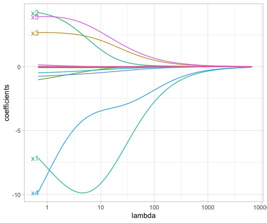
3.2 LASSO regression
The LASSO (least absolute shrinkage and selection operator) penalty (Tibshirani 1996) is a true feature selection method since some variable coefficients will be “pushed” to zero thereby eliminating them from the model.
Mathematically:
\[\min(SSE + \lambda \sum_{j=1}^j \vert\beta_{j}\vert)\]The \(\lambda\) is called the tuning parameter and determines how strong the penalty will affect the coefficient estimates.
The \(\vert\beta_{j}\vert\) term increases the penalty term every time a coefficient is added to the model.
Here is an illustration (Figure 6.3) based on a LASSO regression from housing data:
cpgs <- df_for_regression %>%
  dplyr::select(- age) %>%       # will be placed in another R object
  as.matrix() %>%                # for glmnet function to work properly, needs a matrix data structure
  na.omit()                      # remove NA values (glmnet has no tolerance for missing values)

age <- df_for_regression %>%
  na.omit() %>%
  dplyr::pull(var = age)

my_lasso <- glmnet::glmnet(x = cpgs,
                           y = age,
                           standardize = FALSE,  # since all our values are between 0 and 1. No scale issue.
                           alpha = 1,            # alpha = 1 performs a LASSO analysis. 0 performs a Ridge analysis.
                           family = "gaussian")

my_lambda_lasso_cv <- glmnet::cv.glmnet(
  x = cpgs,
  y = age,
  alpha = 1,
  nfolds = 10,
  lambda = NULL,
  type.measure = "mse")
plot(lambda_lasso, main = "Lasso penalty choice\n\n")
8. References
8.1 Online books and tutorials
- Bradley Boehmke Hands-on Machine Learning with R book sections on regressions:
8.2 Publications and books
- LASSO regression: Hastie, T., R. Tibshirani, and M. Wainwright. 2015. Statistical Learning with Sparsity: The Lasso and Generalizations. Chapman & Hall/Crc Monographs on Statistics & Applied Probability. Taylor & Francis.
- Gareth James, Daniela Witten, Trevor Hastie and Robert Tibshirani. 2013. An Introduction to Statistical Learning Link
Key Points