Advanced Data Exploration on dataset #2
Overview
Teaching: 30 min
Exercises: 30 minQuestions
Table of Contents
- 1. Data exploration
- 2. Finding the differential CpG sites
- 3. Heatmap of the differential CpG
- 4. Exercise
- References
1. Data exploration
1.1 First steps
First things first. Let’s download and import the CpG beta values into R.
download.file(url = "https://zenodo.org/record/4056406/files/cpg_methylation_beta_values.tsv?download=1",
              destfile = "data/cpg_methylation_beta_values.tsv",
              method = "wget",
              quiet = TRUE)


df_cpg <- read.delim("data/cpg_methylation_beta_values.tsv",
                      header = TRUE,
                      stringsAsFactors = FALSE)
Question
- Can you show the first 5 rows and 5 columns?
- How many CpG sites are being investigated?
- How many different samples?
Solution
df_cpg[1:5,1:5]nrow(df_cpg)ncol(df_cpg
We can then download and import the age to sample correspondence into R.
download.file(url = "https://zenodo.org/record/4056406/files/cpg_methylation_sample_age.tsv?download=1",
              destfile = "data/cpg_methylation_sample_age.tsv",
              method = "wget",
              quiet = TRUE)

# Import sample to age correspondence
sample_age <- read.delim("data/cpg_methylation_sample_age.tsv",
                          header = TRUE,
                          stringsAsFactors = FALSE)
1.2 Number and distribution of beta values
Question
Are the number of CpG per sample comparable?
Solution
Yes absolutely. In fact, there are exactly 27,578 CG sites measured for each sample.
df_cpg_tidy %>% group_by(sample) %>% tally() %>% summary()
Since the beta values arise from a microarray hybridization, there is always a signal associated to each CpG probe set. Some signals might be filtered but usually each probe get assigned a value.
Question
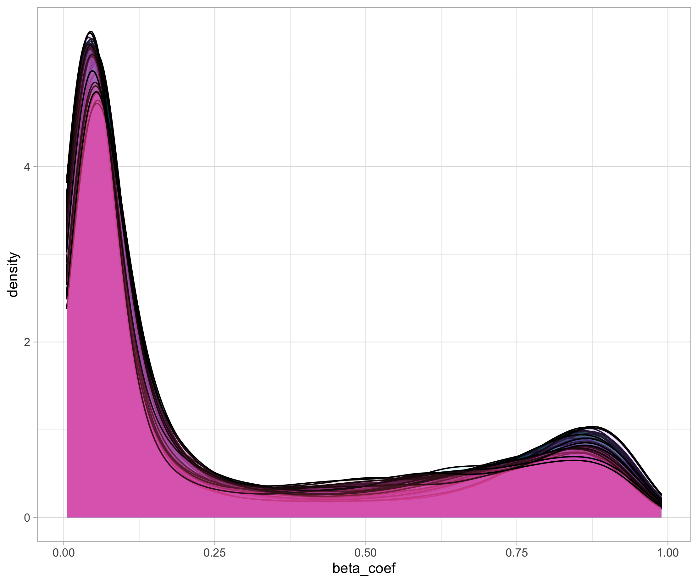
Can you make a density plot to show the distribution of beta values across the different samples? Overlay all density curves so you can see if one sample is very different from the others (possible outlier).
Solution
df_cpg_tidy %>%
  ggplot(data = ., aes(x = beta_coef, fill = sample)) +
      geom_density(alpha = 0.1) +
      guides(fill = FALSE)
This is what you should see:
2. Finding the differential CpG sites
As a way to represent CpG methylation values, a heatmap of CpG beta values clustered on both samples and CpG could reveal groups of CpG islands related to samples of the same age. This would be our first attempt to relate age to methylation values. Yet, we need to take it a step backward because…
Discussion
What could be a potential issue when creating a heatmap based on the complete set of CpG values?
As we have thousands of CpGs, this would create a massive probably uninformative heatmap. Instead, we could keep the CpGs that shows contrasted methylation values across the different samples. Non-differential CpG islands would unlikely to be related to age differences.
2.1 Data massage
First, we need to add the age to each sample to the df_cpg_tidy tibble.
# left join to add age to each sample using the "sample" column as common key
df_cpg_tidy_with_age =  dplyr::left_join(df_cpg_tidy,
                                         sample_age,
                                         by  = "sample")


df_cpg_tidy_with_age
You should get the following output:
# A tibble: 1,820,148 x 8
   CpG_id     sample    beta_coef title source         pair race    age
   <chr>      <chr>         <dbl> <int> <chr>         <int> <chr> <int>
 1 cg00000292 GSM712302     0.790   111 saliva sample     1 White    40
 2 cg00000292 GSM712303     0.684   112 saliva sample     1 White    40
 3 cg00000292 GSM712306     0.766   811 saliva sample     8 White    39
 4 cg00000292 GSM712307     0.821   812 saliva sample     8 White    39
 5 cg00000292 GSM712308     0.633   911 saliva sample     9 White    39
 (... more lines ...)
If you would have only one CpG, this would be easy right? Let’s see how easy!
Question
Can you perform a one-way ANOVA on the “cg00000292” CpG island?
Hint1: Useageas the Y response variable andbeta_coefas the explanatory X variable?
Hint2: usesummary(my_aov_model)to display the related ANOVA p-value.Solution
One approach to do this would be:
 df_cpg_tidy_with_age %>%
   filter(CpG_id == "cg00000292") %>%
   with(data = ., aov(age ~ beta_coef)) %>%
   summary()
It gives the following output: ~~~ Df Sum Sq Mean Sq F value Pr(>F) beta_coef 1 154 154.09 1.99 0.163 Residuals 64 4955 77.42
To do this, the issue is that we need to perform a one-way ANOVA between using the age as the response variable (the Y) and each CpG island methylation values as the X explanatory variable. There, we need to perform….27,568 ANOVAs!
That’s really a lot of tests but we can rely on the List Column Workflow also called the Nest Map Unest strategy to do this. Try to understand the code below and if too complicated, simply execute it:
2.2 Multiple one-factor ANOVAs
Now the piece de resistance to perform the multiple ANOVAs all at once:
fits <- df_cpg_tidy_with_age %>%
  nest(.data = ., - CpG_id) %>%                                                  # categorical variable used for ANOVA
  mutate(fit = map(data, ~ aov(data = ., formula = .$age ~ .$beta_coef))) %>%    # One-factor ANOVA with age as the Y and beta value as X
  mutate(res = map(fit, glance)) %>%                                             # Use broom::glance to return a tibble from a aov/lm object
  unnest(res)
2.3 Detailed explanation
Optional reading
If this section is too complex, feel free to skip it and move to the next section.
Nesting: The nest(.data = ., - CpG_id) line reads the tidy dataframe and perform a nest operation placing all data related to a single CpG island on a single row. There are only two columns, the CpG_id column and another special column called data.
Try the following code:
df_cpg_tidy_with_age %>% nest(.data = ., - CpG_id)

# A tibble: 27,578 x 2
   CpG_id     data
   <chr>      <list>
 1 cg00000292 <tibble [66 × 7]>
 2 cg00002426 <tibble [66 × 7]>
 3 cg00003994 <tibble [66 × 7]>
The data column contains all info related to a single CpG island. For instance try this:
test <- df_cpg_tidy_with_age %>% nest(.data = ., - CpG_id)
test$data[test$CpG_id == "cg00000292"]
This will display the content of the list stored in the data column related to CpG island cg00000292.
[[1]]
# A tibble: 66 x 7
   sample    beta_coef title source         pair race    age
   <chr>         <dbl> <int> <chr>         <int> <chr> <int>
 1 GSM712302     0.790   111 saliva sample     1 White    40
 2 GSM712303     0.684   112 saliva sample     1 White    40
 3 GSM712306     0.766   811 saliva sample     8 White    39
Mapping: Mapping is the action of applying a function to a list for instance. Here we will map the aov() function to each list item stored in the special data column.
df_cpg_tidy_with_age %>%
  nest(.data = ., - CpG_id) %>%
  mutate(fit = map(data, ~ aov(data = ., formula = .$age ~ .$beta_coef)))
The dplyr::mutate() function will add a new column named fit to the tibble. Then the map function will perform a one-way ANOVA on the data special column. It will use age as the response variable and beta_coef as the explanatory variable.
# A tibble: 27,578 x 3
   CpG_id     data              fit
   <chr>      <list>            <list>
 1 cg00000292 <tibble [66 × 7]> <aov>
 2 cg00002426 <tibble [66 × 7]> <aov>
 3 cg00003994 <tibble [66 × 7]> <aov>
The <aov> indicates that we have ANOVA models stored for each CpG island in the fit column.
Unnesting: To extract our results as a normal tibble, we need to unnest the fit column which contains list items and extract it as rows and columns.
This is what the following piece of code does:
fits <- df_cpg_tidy_with_age %>%
  nest(.data = ., - CpG_id) %>% # categorical variable used for ANOVA
  mutate(fit = map(data, ~ aov(data = ., formula = .$age ~ .$beta_coef))) %>%
  mutate(res = map(fit, glance)) %>%
  unnest(res)
There is one extra step because the <aov> data structure is a bit peculiar and does not work well as a dataframe. We therefore use the glance() function from the broom package to do this. We create a new column for this called res that will store our result temporarily. The corresponding R code is mutate(res = map(fit, glance)).
Finally, we can unnest the res column that contains our desired one-way ANOVA results (including ANOVA p-values).
# A tibble: 27,578 x 14
   CpG_id data  fit   r.squared adj.r.squared sigma statistic p.value    df logLik   AIC   BIC deviance
   <chr>  <lis> <lis>     <dbl>         <dbl> <dbl>     <dbl>   <dbl> <int>  <dbl> <dbl> <dbl>    <dbl>
 1 cg000… <tib… <aov>  0.0302         0.0150   8.80   1.99     0.163      2  -236.  478.  485.    4955.
 2 cg000… <tib… <aov>  0.0105        -0.00500  8.89   0.677    0.414      2  -237.  480.  486.    5055.
 3 cg000… <tib… <aov>  0.0301         0.0149   8.80   1.98     0.164      2  -236.  478.  485.    4955.
 4 cg000… <tib… <aov>  0.0531         0.0383   8.69   3.59     0.0628     2  -235.  477.  483.    4838.
 5 cg000… <tib… <aov>  0.000256      -0.0154   8.93   0.0164   0.899      2  -237.  480.  487.    5108.
As you can see, all CpG sites are present since our tibble exhibits 27,578 rows. Each CpG site thus has a associated p-value in the p.value column.
Let’s use this info to filter our df_cpg_tidy_with_age.
2.4 Filtering non-differential CpG sites
Since we performed more than 27,000 one-way ANOVAs, we need to correct for type I error (false positives). We can add a column named fdr for false discovery rate that will contain adjusted p-values.
There are several methods to correct for type I error which can be “bonferroni” (most stringent) or “hochberg” (more relaxed). It goes beyond the scope of this lesson so we will choose one i.e. “hochberg” but feel free to explore: type p.adjust.methods in the R console to show a list of possible methods.
fits_with_fdr <- fits %>%
  mutate(fdr = p.adjust(p.value, method = "hochberg"))

# Threshold of 5% false discovery rate
cpg_differentials <- filter(fits_with_fdr, fdr < 0.05) %>%
  dplyr::pull(CpG_id)

length(cpg_differentials)
We have 228 differential CpGs which should will be easier to display all together on the same heatmap.
Let’s pull out all CpG sites that are differential. This can be achieved rather simply with dplyr filter() and pull(). The latter function takes a tibble column and returns a vector (simpler data structure).
cpg_differentials <- filter(fits, p.value < 0.05) %>%
                     dplyr::pull(CpG_id)

head(cpg_differentials)
"cg00021527" "cg00037940" "cg00054706" "cg00055233" "cg00059225" "cg00080012"
We can now use this vector of differential CpG sites to filter out the “main” dataframe.
df_cpg_tidy_with_age_filtered <- filter(df_cpg_tidy_with_age,
                                        CpG_id %in% cpg_differentials)

# Sanity check: do you find back 228 unique CpG sites?
length(unique(df_cpg_tidy_with_age_filtered$CpG_id))
If you find 228 unique CpG sites with the FDR hochberg correction, then you’re good to go!
3. Heatmap of the differential CpG
Now that with have a nice usable tibble with only differential CpG sites, let’s create the heatmap.
3.1 First version of the heatmap
df_for_heatmap <- pivot_wider(df_cpg_tidy_with_age_filtered,
                              id_cols = CpG_id,
                              names_from = "sample",
                              values_from = "beta_coef") %>%
  column_to_rownames("CpG_id")
This is how it looks like.
df_for_heatmap[1:5,1:5]
           GSM712302  GSM712303  GSM712306  GSM712307 GSM712308
cg00059225 0.3232136 0.36157080 0.34965740 0.35154480 0.4328789
cg00083937 0.5869906 0.61236270 0.61208990 0.50702600 0.7512166
cg00090147 0.0933590 0.09505562 0.07671635 0.08565685 0.1023634
cg00107187 0.1037067 0.12210180 0.11644700 0.11337940 0.1568705
cg00201234 0.2174944 0.23351220 0.19471140 0.21341510 0.3491383
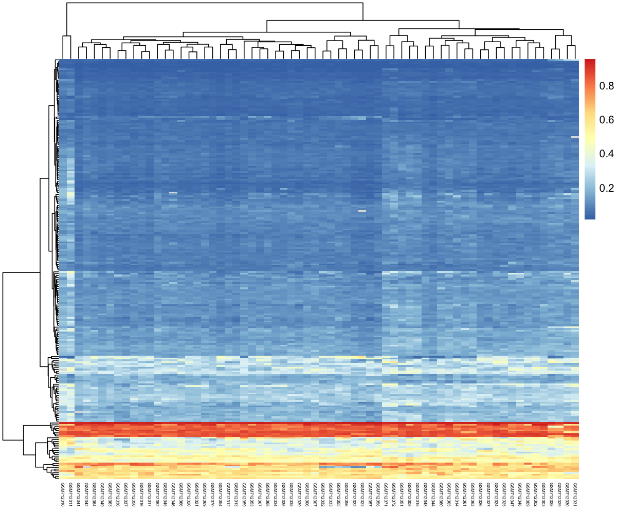
We create the heatmap using the pheatmap() function from the pheatmap package. It has many different options. A convenient way to visualise it is to look at its documentation online here.
my_heatmap <- pheatmap(df_for_heatmap,
                       show_colnames = TRUE,   # sample names
                       show_rownames = FALSE,  # CpG identifiers (not very useful to show so hidden)
                       cluster_rows = TRUE,    # group similar CpG sites together
                       cluster_cols = TRUE,    # group similar samples together
                       fontsize_col = 4)       # to display sample names
3.2 Slight upgrade
One way to dig into our data would be to add the sample age on top of the heatmap.
sample_annot <- sample_age %>% column_to_rownames("sample") %>% select(age)

my_heatmap <- pheatmap(df_for_heatmap,
                       annotation_col = sample_annot,
                       show_colnames = TRUE,
                       show_rownames = FALSE,
                       cluster_rows = TRUE,
                       cluster_cols = TRUE,
                       fontsize_col = 4)
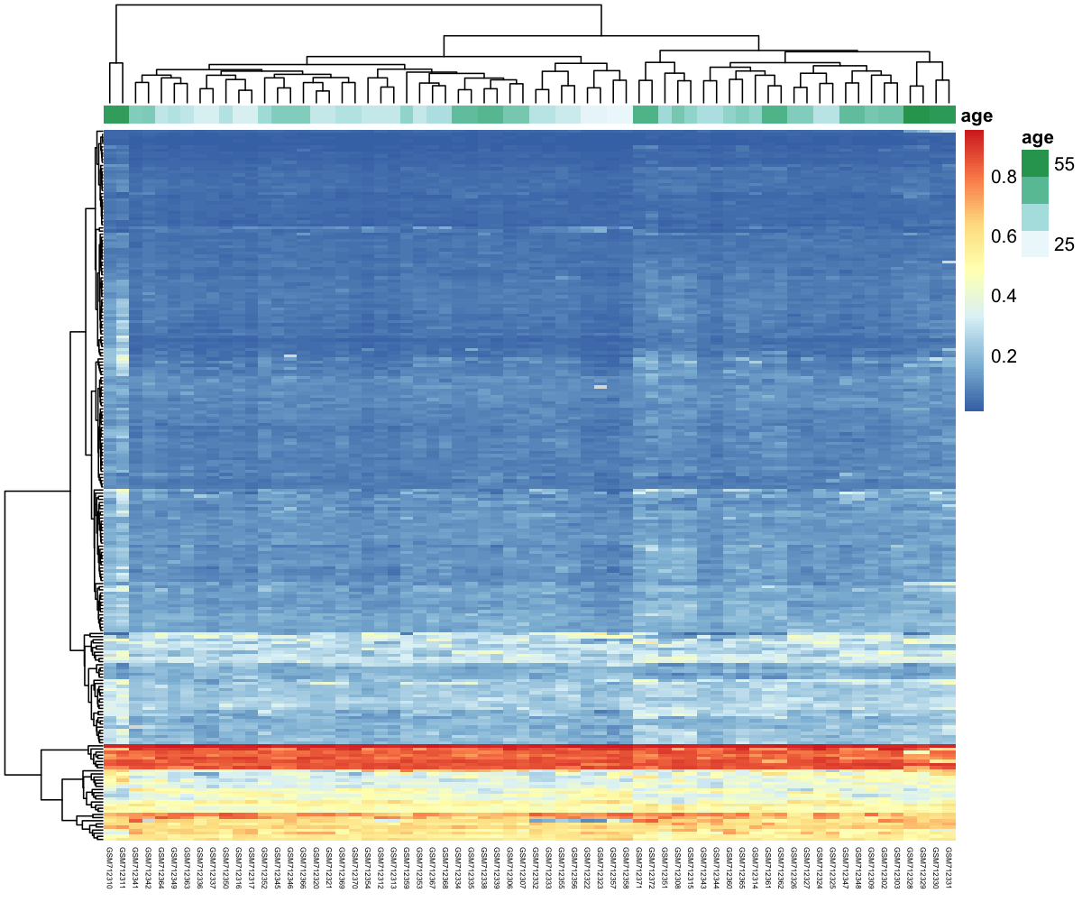
Discussion
How easy is it to find groups of CpG sites related to high ages?
3.3 Saving image on your hard drive
If you want to save your heatmap to an image file on your machine, you can use this helper function.
save_pheatmap_png <- function(x, filename, width=1200, height=1000, res = 150) {
  png(filename, width = width, height = height, res = res)
  grid::grid.newpage()
  grid::grid.draw(x$gtable)
  dev.off()
}

save_pheatmap_png(my_heatmap, "heatmap.png")
3.4 Saving the filtered tidy CpG dataset for the next episodes
# filter out unnecessary columns
# comply with wide format (same as original one but with only 228 CpG sites)
final_df <-
  df_cpg_tidy_with_age_filtered %>%
  dplyr::select(CpG_id, sample, beta_coef) %>%
  pivot_wider(id_cols = sample, names_from = CpG_id, values_from = beta_coef)


# make it wide to comply with the original data format
write.table(x = final_df,
            file = "data/differential_cpgs.tsv",
            quote = FALSE,
            sep = "\t")
4. Exercise
Exercise
Here, a one-way ANOVA was used to test the relationship between CpG site methylation level and age.
- On which hypothesis the one-way ANOVA did rely?
- Can you test some or all of these hypotheses using R?
- If these assumptions are not met, find the equivalent of a one-way ANOVA among non-parametric tests. You can search for
non-parametric ANOVAin your favorite web search engine.
References
- The
broom()package documentation - A vignette to demonstrate the use of
dplyr,broomandmapaltogether to perform nested computations: Link
Key Points