07 Functional enrichment analysis
Overview
Teaching: 60 min
Exercises: 15 minQuestions
Given a list of differentially expressed genes, how do I search for enriched functions?
What is the difference between an over-representation analysis (ORA) and a gene set enrichment analysis (GSEA)?
Objectives
Add extensive gene annotations using Ensembl API queried using the
biomartrpackage.Be able to perform an over representation analysis (ORA) using a list of differentially expressed genes.
Be able to perform a gene set enrichment analysis (GSEA) using a list of differentially expressed genes.
Build graphical representations from the results of an ORA or GSEA analysis.
Table of Contents
- 1. Introduction
- 2. Gene Ontology ORA analysis using AgriGO (webtool)
- 3. Gene Ontology ORA analysis using clusterProfiler (R code)
- 4. Gene Ontology ORA using InterProScan and AgriGO
- 5. KEGG Over Representation Analysis using clusterProfiler (R code)
- 6. KEGG ORA analysis for species without a KEGG classification
- 7. Gene Set Enrichment Analysis (GSEA) with ClusterProfiler
- 8. Going further
1. Introduction
1.1 From a list of genes to biological insights
You’ve finally managed to extract a list of differentially expressed genes from your comparison. Great job!
But…now what? ![]()
![]()
Why did you do the experiment in the first place? Probably because you had an hypothesis or you were looking to open new leads.
A functional enrichement analysis will determine whether some functions are enriched in your set of differentially expressed genes.
In this tutorial, we are looking for Arabidopsis leaf genes that are induced or repressed upon inoculation by Pseudomonas syringae DC3000 after 7 days.
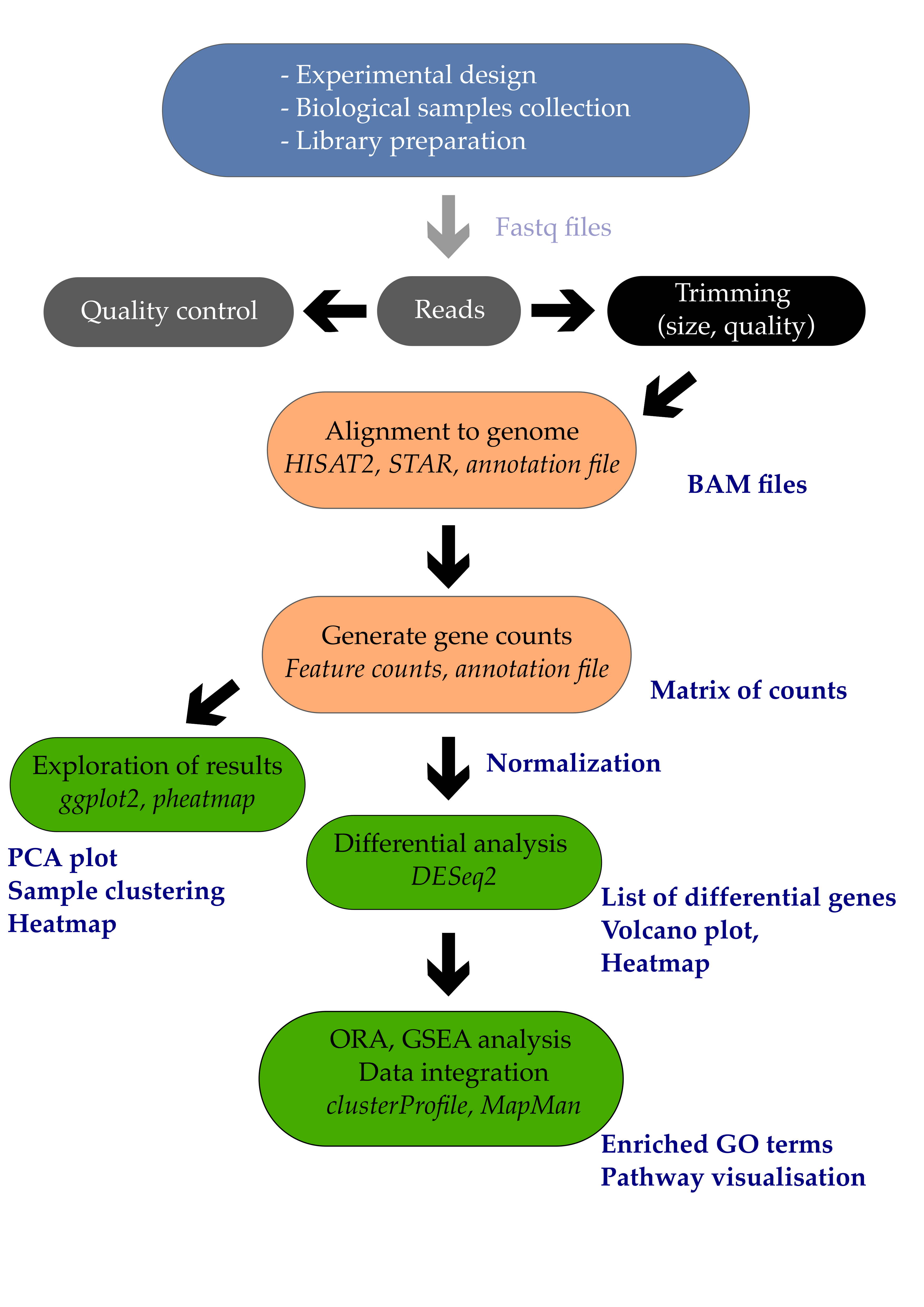
One important goal is to gain a higher view and not only deal with individual genes but understand which pathways are involved in the response.
Once we obtain a list of genes, we have multiple analysis to perform to go beyond a simple list of genes:
- Annotating our list of genes with cross-databases identifiers and descriptions (Entrezid, Uniprot, KEGG, etc.).
- Performing Over-Representation Analysis (ORA) or Gene Set Enrichment Analysis (GSEA) using R or webtools.
- Interpreting the results.
These ORA and GSEA analysis require the use of external resources to assign functions to genes. Two resources are of particular importance and will be examined in this tutorial.
1.2 Over Representation Analysis (ORA)
Over Representation Analysis is searching for biological functions or pathways that are enriched in a list obtained through experimental studies compared to the complete list of functions/pathways.
Usually, ORA makes use of so-called gene ontologies (abbreviated GO) where each gene receives one or multiple layers of information on their function, cellular localization, etc.
The ORA analysis rely on this mathematical equation to compute a p-value for a given gene set classified under a certain GO.
Source: Wikipedia
\[p = 1 - {\sum_{i=0}^{k-1} {M \choose i}{N - M \choose n - i} \over {N \choose n}}\]In this formula:
- N is the total number of genes in the background distribution. Also called the “universe” of our transcriptome.
- M is the number of genes within that distribution that are annotated (either directly or indirectly) to the gene set of interest.
- n is the size of the list of genes of interest (the size of your “drawing”).
- k is the number of genes “drawn” within that list which are annotated to the gene set.
The background distribution by default is by default all genes that have annotation. You can change it to your specific background if you have a good reason for that (only genes with a detectable expression in your expression for instance). Also, p-values should be adjusted for multiple comparison.
Do you remember your math classes from high school? Now’s the time to get them to work again!
Binomial coefficient is defined as \({n \choose k}\) and is equal to \(n! \over {k! (n-k)!}\)
——— drawing of balls from an urn ——
See this great chapter from Prof. Guangchuang Yu (School of Basic Medical Sciences, Southern Medical University, China) for more info.
1.3 The Gene Ontology (GO) resource
The Gene Ontology (GO) produces a bird’s-eye view of biological systems by building a tree of terms related to biological functions. This is particularly helpful when dealing with results from genome-wide experiments (e.g. transcriptomics) since classifying genes into groups of related functions can assist in the interpretation of results. Rather than focusing on each gene, one by one, the researcher gets access to metabolic pathways, functions related to development, etc.
Note
The GO resource is divided into 3 main subdomains:
- Biological Process (BP): a series of molecular events with a defined beginning and end relevant for the function of an organism, a cell, etc.
- Cellular Component (CC): the part of a cell.
- Molecular Function (MF): the enzymatic activites of a gene product.
Source Wikipedia.
Let’s take an example. The At3g53260 gene codes for a phenylalanine ammonia-lyase (PAL) that catalyses the following reaction and is one of the first step of cell wall synthesis, flavonoid synthesis, etc. ; L-phenylalanine ⇌ trans-cinnamic acid + \(NH_{3}\)
This gene has several GO terms associated:
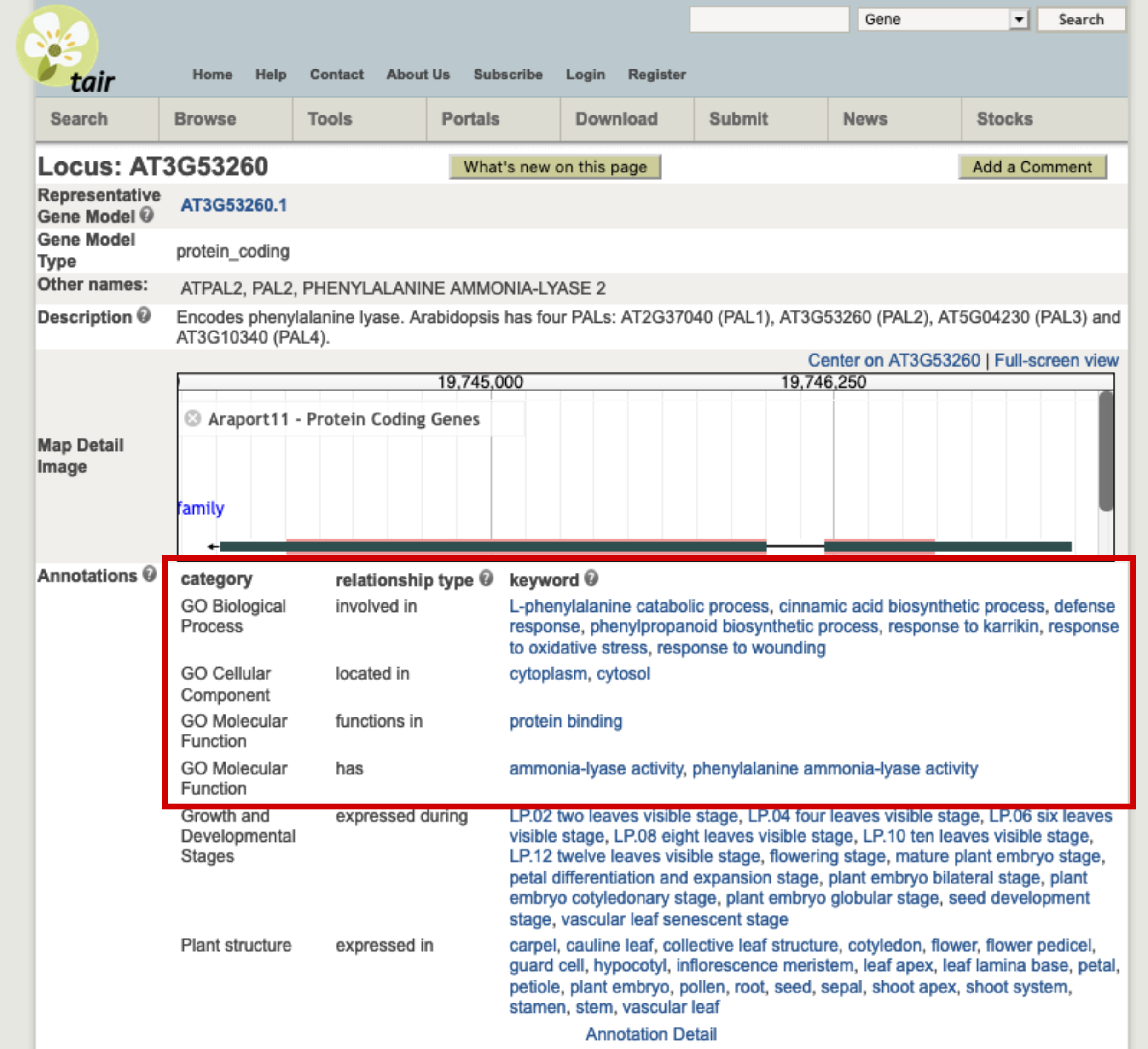
Here are an example term associated with each GO subdomain:
- BP: the “L-phenylalanine catabolic process” term with the GO:0006559 unique identifier.
- CC: the “cytoplasm” term with the GO:0005737 unique identifier.
- MF: the “ammonia-lyase activity” term with the GO:0016841 unique identifier.
Exercise
Go to the AmiGO 2 website and enter the term “GO:0006559” (L-phenylalanine catabolic process).
- Can you find the number of genes in ALL organisms that are associated with this term?
- Can you find the number of genes ONLY in Arabidopsis thaliana associated with this term?
Solution
- There are 712 genes in all organisms associated with this term (AmiGO 2 version 2.5.13). Hint: Using the free text filter field and “arabidopsis thaliana pal1”, you rapidly find that PAL1 has the AT2G37040 gene identifier.
- There are 12 genes associated with this term in Arabidopsis thaliana. By clicking on “Organism” and filtering to keep only “Viridiplantae” species, one can see 12 genes next to Arabidopsis.
1.4 The Kyoto Encyclopedia of Genes and Genomes (KEGG) database
KEGG stands for the “Kyoto Encyclopedia of Genes and Genomes”. From the KEGG website home page:
KEGG is a database resource for understanding high-level functions and utilities of the biological system, such as the cell, the organism and the ecosystem, from molecular-level information, especially large-scale molecular datasets generated by genome sequencing and other high-throughput experimental technologies.
Instead of using the Gene Ontology gene classification, one might be interested to use KEGG classification to view the transcriptomic response of an organism. KEGG is not restricted to metabolic functions but has a great deal of metabolic maps that can help you.
Important note
While using a model organism such as Arabidopsis thaliana makes ORA and GSEA analyses easier, it is noteworthy that the GO and KEGG resources are not restricted to model organisms but rather include a huge number of (plant) species.
2. Gene Ontology ORA analysis using AgriGO (webtool)
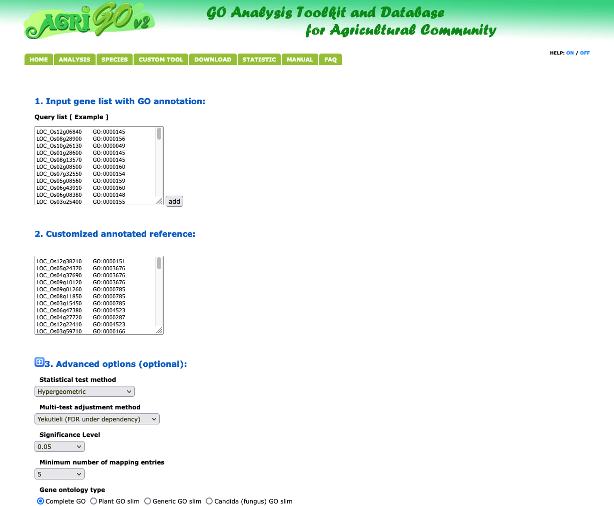
AgriGO v2.0 is a webtool accessible here to perform gene ontology analyses. Two papers describe it extensively (see 8.2. References).
From the AgriGO v2.0 home page:
AgriGO v2.0 is a web-based tool and database for gene ontology analyses. It specifically focuses on agricultural species and is user-friendly. AgriGO v2.0 is designed to provide deep support to the agricultural community in the realm of ontology analyses.
You can find an extensive manual available here to guide you through the main steps.
Important note
There are two versions of AgriGO currently online, versions 1.x and version 2.0. Make sure you go to the latest 2.0 version url.
Agrigo Alternatives for other organisms
Agrigo is developed for agricultural data, as the name suggests. If you are working human or animal data there are alternative webtools that can be used. For example Panther. This works with similar gene ID input.
2.1 Read and import differential genes
diff_genes <- read_delim(file = "differential_genes.tsv", delim = "\t")
You can check that you have imported the 4979 differentially expressed genes.
nrow(diff_genes)
[1] 4979
2.2 Single Enrichment Analysis
We can perform a Single Enrichment Analysis (SEA) which is essentially similar to an ORA. AgriGO supports species-specific analyses.
For Arabidopsis thaliana navigate here.
First, write gene identifiers to a text file from which you can copy-paste the identifiers. Here, we use the complete list of the 4979 genes differentially regulated (DC3000 versus Mock) but you can filter it on some criteria (e.g. fold change). This is what I’ve done to gather less genes and speed up the SEA analysis.
diff_genes %>%
  filter(log2FoldChange > 0) %>%
  with(.,quantile(log2FoldChange, c(0.5,0.75,0.9)))

diff_genes %>%
  filter(log2FoldChange > quantile(log2FoldChange, c(0.75))) %>% # keeping fold changes above the 75th percentile
  dplyr::select(genes) %>%
  write.table(., file = "diff_genes_for_agrigo.tsv", row.names = FALSE, quote = FALSE)
Open this list using a text editor and copy-paste it into the “input a gene list” box.
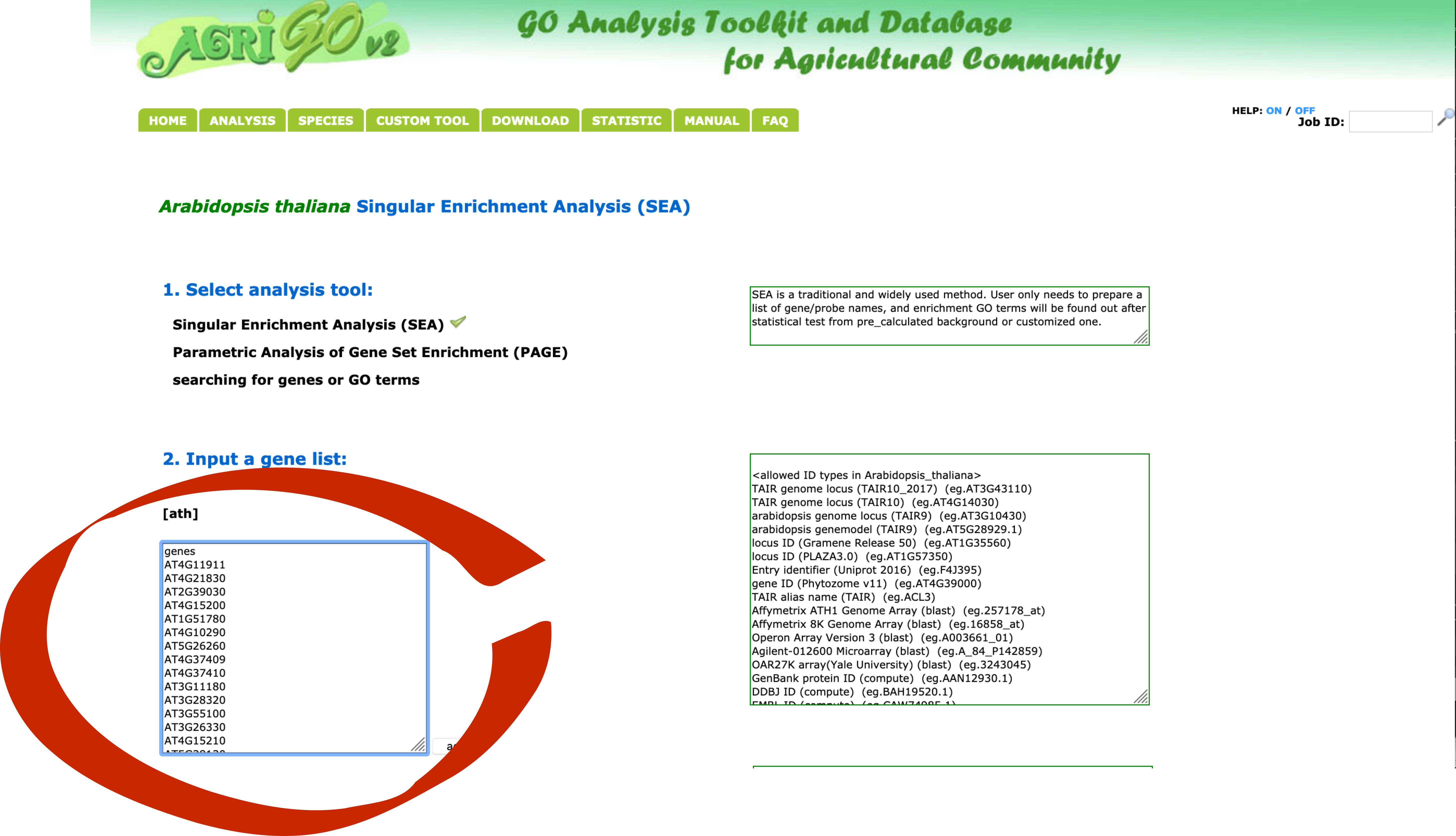
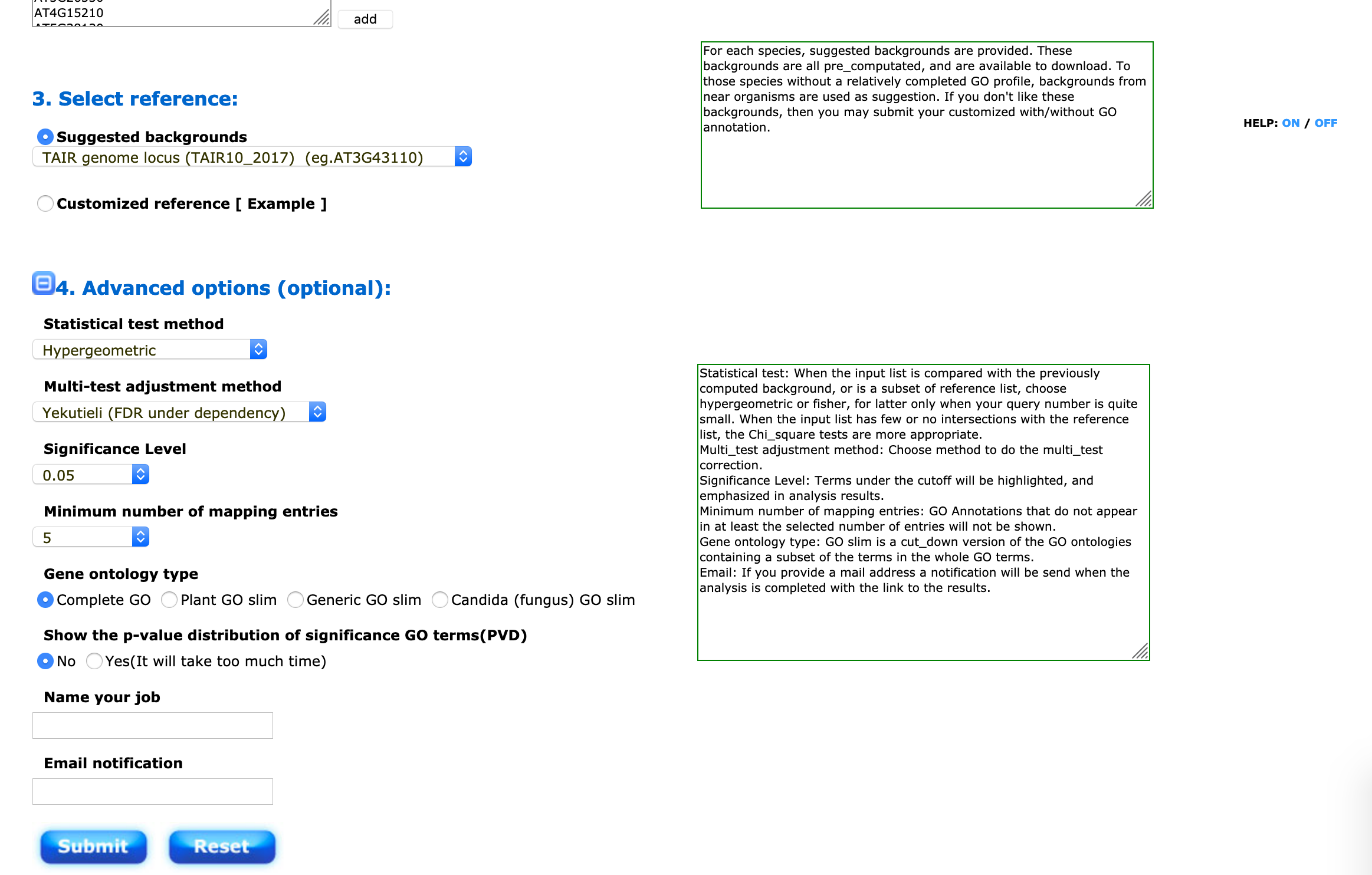
You will then have to choose a background (your “universe”) to perform the SEA/ORA analysis. For Arabidopsis thaliana, you can choose the suggested background (TAIR10).
This step is exactly the same for Panther with other organisms.
I suggest to use the hypergeometric distribution and the Yekutieli False Discovery Rate correction. The significance threshold and the minimum number of entries can be changed depending on the size of your input gene list.
If you have a long list, you might write your email address to collect your results later (analysis might take a while). You will arrive on a result page from which you can generate graphs, barplots, tables etc.

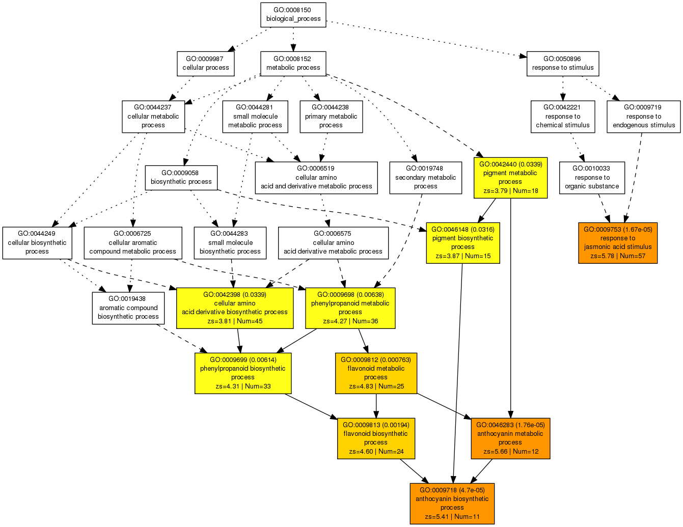
This DAG view gives a comprehensive overview of the GO terms and their relationships.
2.3 Parametric Analysis of Gene Set Enrichment
This analysis takes expression values also into account and could be an richer alternative to SEA.
diff_genes %>%
  filter(log2FoldChange > quantile(log2FoldChange, c(0.75))) %>%
  dplyr::select(genes, log2FoldChange) %>%
  write.table(., file = "diff_genes_for_agrigo_page.tsv", sep = "\t", row.names = FALSE, quote = FALSE)
3. Gene Ontology ORA analysis using clusterProfiler (R code)
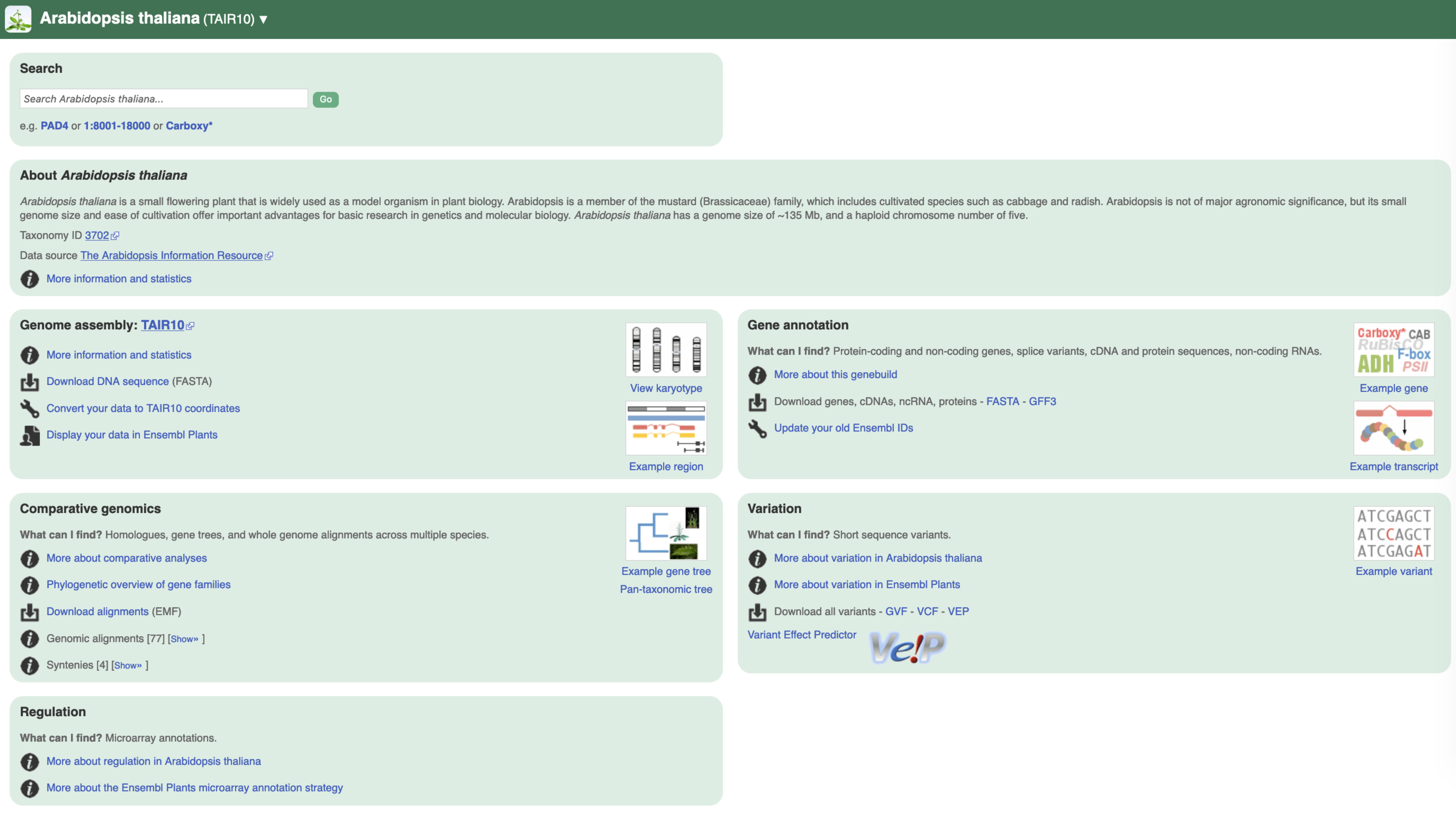
This section can be used for non-model species that have genomic information Ensembl. At the time of writing (November 2021), there are 114 plant species available on EnsemblPlants.
Gene information can be automatically queried directly from R to access the Ensembl databases. Ensembl gathers a tremendous amount of genomic information which can be accessed through a web browser or programmatically.
The Ensembl (https://www.ensembl.org) is a system for generating and distributing genome annotation such as genes, variation, regulation and comparative genomics across the vertebrate subphylum and key model organisms. The Ensembl annotation pipeline is capable of integrating experimental and reference data from multiple providers into a single integrated resource. Here, we present 94 newly annotated and re-annotated genomes, bringing the total number of genomes offered by Ensembl to 227.
We are going to use two fantastic resources: the Ensembl database and the biomartr package. Together, they will automate a lot of tedious and tiring steps when you want to retrieve gene annotations, sequences, etc.
This step is meant to retrieve the correspondence between organism-specific gene identifiers (e.g. At1g01020) and NCBI Entrez Gene ID (e.g. 839321) which are used by clusterProfiler.
We are going to load the required library first.
library("biomartr")
library("clusterProfiler")
library("tidyverse")
library("enrichplot")
suppressPackageStartupMessages(library("org.At.tair.db"))
library("biomaRt")  # only use to remove cache bug
Important note: troubleshooting
If biomart refuses to query Ensembl again, run this command:
biomaRt::biomartCacheClear() # to solve a known bug https://github.com/BioinformaticsFMRP/TCGAbiolinks/issues/335This will clean the cache memory and allow to perform the Ensembl query again.
3.1 Load the table of differential genes
If not done yet, load the table of differential genes.
diff_genes <- read_delim(file = "differential_genes.tsv", delim = "\t")
All what we know about the differential genes are their locus identifier. Not much…. We are missing functional information which we will add.
3.2 Annotating your DE genes with Ensembl and biomartr
What purpose serves biomartr? From the documentation:
The first step, however, of any genome based study is to retrieve genomes and their annotation from databases. To automate the retrieval process of this information on a meta-genomic scale, the biomartr package provides interface functions for genomic sequence retrieval and functional annotation retrieval. The major aim of biomartr is to facilitate computational reproducibility and large-scale handling of genomic data for (meta-)genomic analyses. In addition, biomartr aims to address the genome version crisis. With biomartr users can now control and be informed about the genome versions they retrieve automatically. Many large scale genomics studies lack this information and thus, reproducibility and data interpretation become nearly impossible when documentation of genome version information gets neglected.
What is available for Arabidopsis thaliana in Ensembl?
# library("biomartr") (if not loaded already)
biomartr::organismBM(organism = "Arabidopsis thaliana")
organism_name description                                                  mart         dataset       version
  <chr>         <chr>                                                        <chr>        <chr>         <chr>
1 athaliana     Arabidopsis thaliana genes (TAIR10)                          plants_mart  athaliana_eg… TAIR10
2 athaliana     Arabidopsis thaliana Short Variants (SNPs and indels exclud… plants_vari… athaliana_eg… TAIR10
This indicates that we can get a dataset called athaliana_eg_gene of the genome annotation version TAIR10 from the plant_mart mart.
Let’s see how many different information fields we can retrieve from the arabidopsis_eg_gene dataset.
arabido_attributes =
  biomartr::organismAttributes("Arabidopsis thaliana") %>%
  filter(dataset == "athaliana_eg_gene")
arabido_attributes
# A tibble: 2,574 x 4
   name                  description              dataset           mart
   <chr>                 <chr>                    <chr>             <chr>
 1 ensembl_gene_id       Gene stable ID           athaliana_eg_gene plants_mart
 2 ensembl_transcript_id Transcript stable ID     athaliana_eg_gene plants_mart
 3 ensembl_peptide_id    Protein stable ID        athaliana_eg_gene plants_mart
 4 ensembl_exon_id       Exon stable ID           athaliana_eg_gene plants_mart
 5 description           Gene description         athaliana_eg_gene plants_mart
 6 chromosome_name       Chromosome/scaffold name athaliana_eg_gene plants_mart
 7 start_position        Gene start (bp)          athaliana_eg_gene plants_mart
 8 end_position          Gene end (bp)            athaliana_eg_gene plants_mart
 9 strand                Strand                   athaliana_eg_gene plants_mart
10 band                  Karyotype band           athaliana_eg_gene plants_mart
# … with 2,564 more rows
![]() There is quite some information in there! We should be able to get what we want = the correspondence between the Arabidopsis gene identifier and the NCBI Entrez Gene identifier.
There is quite some information in there! We should be able to get what we want = the correspondence between the Arabidopsis gene identifier and the NCBI Entrez Gene identifier.
attributes_to_retrieve = c("tair_symbol", "entrezgene_id")

result_BM <- biomartr::biomart( genes      = diff_genes$genes,                  # genes were retrieved using biomartr::getGenome()
                                mart       = "plants_mart",                     # marts were selected with biomartr::getMarts()
                                dataset    = "athaliana_eg_gene",               # datasets were selected with biomartr::getDatasets()
                                attributes = attributes_to_retrieve,            # attributes were selected with biomartr::getAttributes()
                                filters =   "ensembl_gene_id" )# query key
head(result_BM)
We now have our original gene identifiers (column ensembl_gene_id) with the retrieved TAIR symbols (tair_symbol) and NCBI Entrez Gene Id (entrezgene_id).
  ensembl_gene_id  tair_symbol entrezgene_id
1       AT1G01030         NGA3        839321
2       AT1G01070                     839550
3       AT1G01090 PDH-E1 ALPHA        839429
4       AT1G01140        CIPK9        839349
5       AT1G01220         FKGP        839420
6       AT1G01225                     839358
For other species
If your species is not “Arabidopsis thaliana”, simply change your R code here:
# library("biomartr") (if not loaded already)
biomartr::organismBM(organism = "[my favorite species]")
This will retrieve the information available for your species on Ensembl.
3.3 ORA with clusterProfiler
To perform the ORA within R, we will use the clusterProfiler Bioconductor package that has an extensive documentation available here.
First, we need to annotate both genes that make up our “universe” and the genes that were identified as differentially expressed.
# building the universe!
all_arabidopsis_genes <- read.delim("counts.txt", header = T, stringsAsFactors = F)[,1] # directly selects the gene column

# we want the correspondence of TAIR/Ensembl symbols with NCBI Entrez gene ids
attributes_to_retrieve = c("tair_symbol", "uniprotswissprot","entrezgene_id")

# Query the Ensembl API
all_arabidopsis_genes_annotated <- biomartr::biomart(genes = all_arabidopsis_genes,
                                                     mart       = "plants_mart",
                                                     dataset    = "athaliana_eg_gene",
                                                     attributes = attributes_to_retrieve,
                                                     filters =  "ensembl_gene_id" )

# for compatibility with enrichGO universe
# genes in the universe need to be characters and not integers (Entrez gene id)
all_arabidopsis_genes_annotated$entrezgene_id = as.character(
  all_arabidopsis_genes_annotated$entrezgene_id)
We now have a correspondence for all our genes found in Arabidopsis.
# retrieving NCBI Entrez gene id for our genes called differential
diff_arabidopsis_genes_annotated <- biomartr::biomart(genes = diff_genes$genes,
                                                     mart       = "plants_mart",
                                                     dataset    = "athaliana_eg_gene",
                                                     attributes = attributes_to_retrieve,
                                                     filters =  "ensembl_gene_id" )
This gave us the second part which is the classification of genes “drawn” from the whole gene universe. The “drawing” is coming from the set of genes identified as differential (see episode 06).
# performing the ORA for Gene Ontology Biological Process class
ora_analysis_bp <- enrichGO(gene = diff_arabidopsis_genes_annotated$entrezgene_id,
                            universe = all_arabidopsis_genes_annotated$entrezgene_id,
                            OrgDb = org.At.tair.db,  # contains the TAIR/Ensembl id to GO correspondence for A. thaliana
                            keyType = "ENTREZID",
                            ont = "BP",              # either "BP", "CC" or "MF",
                            pAdjustMethod = "BH",
                            qvalueCutoff = 0.05,
                            readable = TRUE,
                            pool = FALSE)
Since we have 3 classes for GO terms i.e. Molecular Function (MF), Cellular Component (CC) and Biological Processes (BP), we have to run this 3 times for each GO class.
Exercise
How many GO categories do you find overrepresented (padj < 0.05) for the Cellular Component and Molecular Function classes?
The Gene Ontology classification is very redundant meaning that parental terms overlap a lot with their related child terms. The clusterProfiler package comes with a dedicated function called simplify to solve this issue.
# clusterProfiler::simplify to disambiguate which simplify() function you want to use
ora_analysis_bp_simplified <- clusterProfiler::simplify(ora_analysis_bp)
The ora_analysis_bp_simplified is a rich and complex R object. It contains various layers of information (R object from the S4 class). Layers can be accessed through the “@” notation.
You can extract a nice table of results for your next breakthrough publication like this.
write_delim(x = as.data.frame(ora_analysis_bp_simplified@result),
            path = "go_results.tsv",
            delim = "\t")

# have a look at a few columns and rows if you'd like.
ora_analysis_bp_simplified@result[1:5,1:8]
           ONTOLOGY         ID                         Description GeneRatio   BgRatio       pvalue     p.adjust       qvalue
GO:0009753       BP GO:0009753           response to jasmonic acid  257/3829 474/20450 1.099409e-68 1.772247e-65 1.160744e-65
GO:0009611       BP GO:0009611                response to wounding  187/3829 335/20450 1.252868e-52 1.009812e-49 6.613824e-50
GO:0006612       BP GO:0006612       protein targeting to membrane  199/3829 374/20450 1.683735e-51 4.690438e-49 3.072032e-49
GO:0010243       BP GO:0010243 response to organonitrogen compound  222/3829 443/20450 1.707866e-51 4.690438e-49 3.072032e-49
GO:0072657       BP GO:0072657    protein localization to membrane  200/3829 377/20450 1.745821e-51 4.690438e-49 3.072032e-49
3.4 Plots from the Gene Ontology ORA analysis
Nice to have all this textual information but an image is worth a thousand words so let’s create some visual representations.
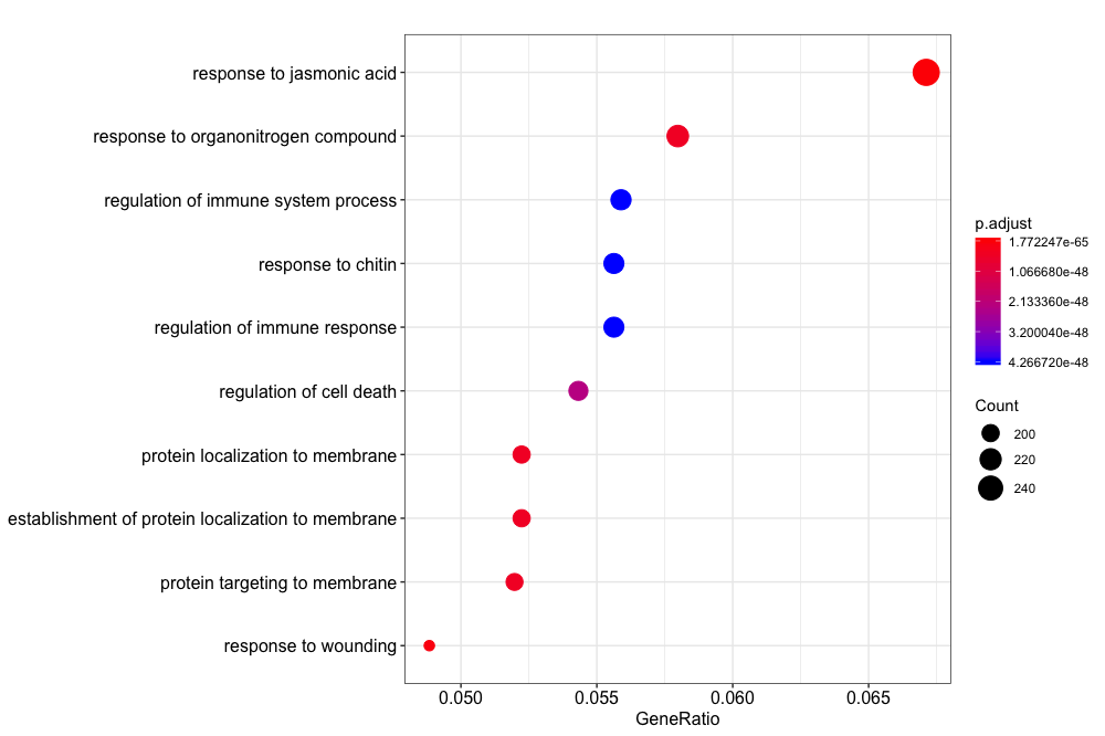
A dotplot can be created very easily.
dotplot(ora_analysis_bp_simplified)
You can also create an enrichment map that connects GO terms with edges between overlapping gene sets. This makes it easier to identify functional modules.
ora_analysis_bp <- pairwise_termsim(ora_analysis_bp, method = "JC")
emapplot(ora_analysis_bp, color = "qvalue")
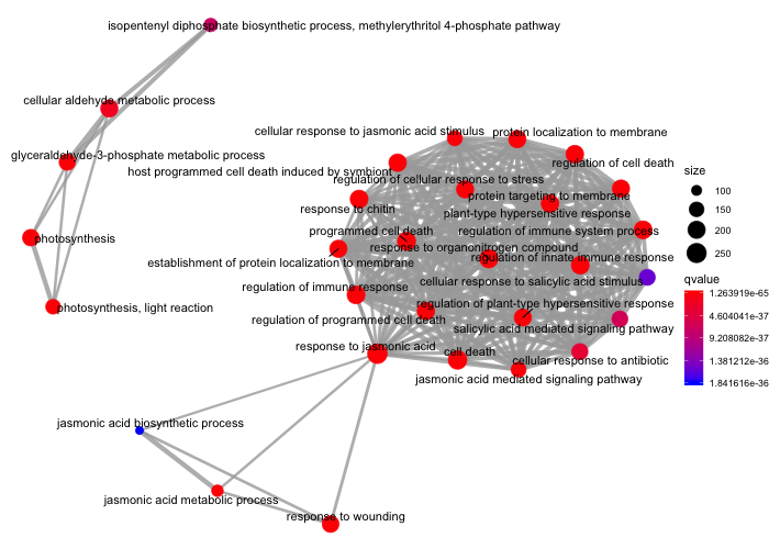
On this plot, we can see that one major module related to cell death, the immune response etc. is to be seen along with two minor modules related to metabolism (upper left) and one related to jasmonic acid and wounding (bottom).
Important note
Remember to perform the analysis for all GO categories:
- Biological Process (
ont = "BP"),- Cellular Component (
ont = "CC"),- Molecular Function (
ont = "MF").
4. Gene Ontology ORA using InterProScan and AgriGO
In this section, we assume that you do not dispose of a Gene Ontology classification of your species genes. Therefore, you will have to obtain it using the predicted protein sequences as a starting point.
4.1 Retrieving protein sequences
For this lesson, we will start from the FASTA file of Arabidopsis thaliana proteins. The ~48,000 proteins predicted from the Arabidopsis genome can be retrieved here.
These are the two first entries of this FASTA file.
>AT1G01010.1 | NAC domain containing protein 1 | Chr1:3760-5630 FORWARD LENGTH=429 | 201606
MEDQVGFGFRPNDEELVGHYLRNKIEGNTSRDVEVAISEVNICSYDPWNLRFQSKYKSRD
AMWYFFSRRENNKGNRQSRTTVSGKWKLTGESVEVKDQWGFCSEGFRGKIGHKRVLVFLD
GRYPDKTKSDWVIHEFHYDLLPEHQRTYVICRLEYKGDDADILSAYAIDPTPAFVPNMTS
SAGSVVNQSRQRNSGSYNTYSEYDSANHGQQFNENSNIMQQQPLQGSFNPLLEYDFANHG
GQWLSDYIDLQQQVPYLAPYENESEMIWKHVIEENFEFLVDERTSMQQHYSDHRPKKPVS
GVLPDDSSDTETGSMIFEDTSSSTDSVGSSDEPGHTRIDDIPSLNIIEPLHNYKAQEQPK
QQSKEKVISSQKSECEWKMAEDSIKIPPSTNTVKQSWIVLENAQWNYLKNMIIGVLLFIS
VISWIILVG
>AT1G01020.1 | ARV1 family protein | Chr1:6915-8666 REVERSE LENGTH=245 | 201606
MAASEHRCVGCGFRVKSLFIQYSPGNIRLMKCGNCKEVADEYIECERMIIFIDLILHRPK
VYRHVLYNAINPATVNIQHLLWKLVFAYLLLDCYRSLLLRKSDEESSFSDSPVLLSIKVL
IGVLSANAAFIISFAIATKGLLNEVSRRREIMLGIFISSYFKIFLLAMLVWEFPMSVIFF
VDILLLTSNSMALKVMTESTMTRCIAVCLIAHLIRFLVGQIFEPTIFLIQIGSLLQYMSY
FFRIV
...etc...
For other species
For your favorite species of interest, you might dispose of a FASTA file with all your proteins. Alternatively, you will have to generate one based on RNA-seq data and a genome reference for instance.
While out of scope for this lesson, please consult the exhaustive Trinity documentation to find a way to obtain a complete protein fasta file.
4.2 InterProScan
Overview
InterProScan is a standalone software that scans protein sequences against a database of protein functions. These are retrieved using information about protein domains.
Provided a FASTA file of protein sequences, one can use InterProScan to retrieve information about the proteins. In detail, InterProScan looks inside these databases:
TIGRFAM (XX.X) : TIGRFAMs are protein families based on Hidden Markov Models or HMMs
SFLD (X.X) : SFLDs are protein families based on Hidden Markov Models or HMMs
amap (XXXXXX.XX) : High-quality Automated and Manual Annotation of Microbial Proteomes
SMART (X.X) : SMART allows the identification and analysis of domain architectures based on Hidden Markov Models or HMMs
CDD (X.XX) : Prediction of CDD domains in Proteins
ProSiteProfiles (XX.XXX) : PROSITE consists of documentation entries describing protein domains, families and functional sites as well as associated patterns and profiles to identify them
ProSitePatterns (XX.XXX) : PROSITE consists of documentation entries describing protein domains, families and functional sites as well as associated patterns and profiles to identify them
SUPERFAMILY (X.XX) : SUPERFAMILY is a database of structural and functional annotation for all proteins and genomes.
PRINTS (XX.X) : A fingerprint is a group of conserved motifs used to characterise a protein family
PANTHER (X.X) : The PANTHER (Protein ANalysis THrough Evolutionary Relationships) Classification System is a unique resource that classifies genes by their functions, using published scientific experimental evidence and evolutionary relationships to predict function even in the absence of direct experimental evidence.
Gene3D (X.X.X) : Structural assignment for whole genes and genomes using the CATH domain structure database
PIRSF (X.XX) : The PIRSF concept is being used as a guiding principle to provide comprehensive and non-overlapping clustering of UniProtKB sequences into a hierarchical order to reflect their evolutionary relationships.
Pfam (XX.X) : A large collection of protein families, each represented by multiple sequence alignments and hidden Markov Models (HMMs)
Coils (X.X) : Prediction of Coiled Coil Regions in Proteins
MobiDBLite (X.X) : Prediction of disordered domains Regions in Proteins
Interproscan installation
To install InterProScan locally on a Linux server, follow the installation instructions.
Specically, you have to run:
mkdir my_interproscan
cd my_interproscan
wget https://ftp.ebi.ac.uk/pub/software/unix/iprscan/5/5.52-86.0/interproscan-5.52-86.0-64-bit.tar.gz
wget https://ftp.ebi.ac.uk/pub/software/unix/iprscan/5/5.52-86.0/interproscan-5.52-86.0-64-bit.tar.gz.md5

# Recommended checksum to confirm the download was successful:
md5sum -c interproscan-5.52-86.0-64-bit.tar.gz.md5
# Must return *interproscan-5.52-86.0-64-bit.tar.gz: OK*
# If not - try downloading the file again as it may be a corrupted copy.
You will probably need a custom installation of Java to make sure you have Java version 11. One way is to install it through conda/mamba. Mamba is a fast re-implementation of conda. For complete info, see this blog post.
wget -O Mambaforge.sh <https://github.com/conda-forge/miniforge/releases/latest/download/Mambaforge-$(uname)-$>(uname -m).sh
bash Mambaforge.sh -b
source mambaforge/bin/activate
Follow the instructions.
To install the Java and Python dependencies of InterProScan, you can run:
mamba install python=3.8 openjdk=11.0.1 -c conda-forge --yes
4.3 Running InterProScan on your proteins
You are now ready to run InterProScan on your FASTA file.
./interproscan.sh -d results_dir/ -goterms -i arabidopsis/Araport11_genes.201606.pep.parsed.fasta --tempdir temp_dir/ --cpu 16 -f TSV -dra --appl PANTHER,Pfam,CDD
Here, the databases searched were restricted to PANTHER, Pfam and the CDD (Conserved Domain Database) to speed up the application.
Some other useful options:
| option short name | option long name | suggestion |
|---|---|---|
| -dp | disable pre-lookup | do not use this option but rather use the precalculated match lookup service. |
| -goterms | look for GO terms | lookup of corresponding Gene Ontology annotation (based on InterPro annotation) |
| -cpu | number of threads | make sure you also have enough memory (RAM) for the number of CPUs choosen |
| -dra | disable residue annotation | prevent InterProScan from calculating the residue level annotations |
CPU and Memory
The more CPU you request, the more memory you will need. See the InterProScan documentation on this point to make sure that you have enough memory to perform the InterProScan run.
Special characters
Make sure that your protein sequences do not have any special characters within their sequence such as “*”. To remove them, you can use Biopython for instance.
from Bio import SeqIO
with open("Araport11_genes.201606.pep.fasta","r") as filin:
    recs = [rec for rec in SeqIO.parse(filin, "fasta")]

with open("Araport11_genes.201606.pep.parsed.fasta", "w") as fileout:
    for rec in recs:
        if "*" in str(rec.seq):
            print("skip this sequence")
    else:
        fileout.write(">" + str(rec.id) + "\n" + str(rec.seq) + "\n")
4.3 Parsing the retrieved GO categories for all proteins
An example result file based on the complete Arabidopsis proteome and from the above InterProScan run is available on Zenodo.
This result file needs to be transformed before we can use it.
interpro <- read.delim("00.tutorial/interproscan_results.tsv", header = F, stringsAsFactors = F, row.names = NULL)

new_colnames <- c("protein_id",
                  "md5",
                  "seq_len",
                  "analysis",
                  "signature_accession",
                  "signature_description",
                  "start",
                  "stop",
                  "score",
                  "status",
                  "date",
                  "interpro_accession",
                  "interpro_description",
                  "go")
colnames(interpro) <- new_colnames

interpro_go <-
  interpro %>%
  dplyr::select(protein_id, go) %>%
  dplyr::filter(go != "-") %>%
  dplyr::filter(go != "")
tail(interpro_go, n = 10)
       protein_id                    go
53735 AT1G79550.2 GO:0004618|GO:0006096
53736 AT3G23700.1            GO:0003676
53737 AT3G23700.1            GO:0003676
53738 AT2G46610.1 GO:0000398|GO:0005681
53739 AT2G46610.1            GO:0003676
53740 AT2G46610.1            GO:0003676
53741 AT5G48560.1            GO:0046983
53742 AT5G48560.1            GO:0006355
53743 AT1G08720.1 GO:0004672|GO:0006468
53744 AT5G57290.3 GO:0003735|GO:0005840
splitted_interpro_go <- cSplit(indt = interpro_go, splitCols = "go", sep = "|", direction = "long")
dedup_go  <- splitted_interpro_go %>% distinct()
tail(dedup_go)
This gives you a nicely formatted dataframe with your genes and their corresponding GO categories (one or more).
    protein_id         go
1: AT5G48560.1 GO:0046983
2: AT5G48560.1 GO:0006355
3: AT1G08720.1 GO:0004672
4: AT1G08720.1 GO:0006468
5: AT5G57290.3 GO:0003735
6: AT5G57290.3 GO:0005840
A few extra things are required to prepare the next steps.
# change column name
dedup_go <- dedup_go %>%
  dplyr::rename("genes" = "protein_id") %>%
  mutate(genes = substr(genes, 1, 9))
tail(dedup_go)
Write to a .csv file for further analysis.
write.csv(x = dedup_go,
          file = "gene_ontologies_all_genes.csv",
          row.names = F)
Universe
This long list of gene identifiers and GO terms is our universe (“the urn”).
4.4 Getting the Gene Ontology ORA analysis
All we need to do now is to retrieve the GO terms for our list of differential genes.
If not done already, import the list of differential genes again:
diff_genes <- read_delim(file = "differential_genes.tsv", delim = "\t")
diff_genes_go <- inner_join(x = dedup_go, y = diff_genes)
head(diff_genes_go)
This gives us the GO term associated with each of our differential gene.
       genes         go   baseMean log2FoldChange      lfcSE      stat       pvalue         padj
1: AT4G26850 GO:0080048 22485.3423      1.2128249 0.17894147  6.777774 1.220414e-11 4.557702e-10
2: AT5G23980 GO:0016491   314.9837     -0.9275218 0.20884912 -4.441110 8.949619e-06 9.361972e-05
3: AT1G70070 GO:0003676  2279.0575     -0.5180395 0.11799985 -4.390171 1.132617e-05 1.150921e-04
4: AT1G70070 GO:0005524  2279.0575     -0.5180395 0.11799985 -4.390171 1.132617e-05 1.150921e-04
5: AT5G66400 GO:0009415  2405.2748     -0.4386227 0.10170489 -4.312700 1.612727e-05 1.562633e-04
6: AT1G54360 GO:0006367   904.5027     -0.2470180 0.06825266 -3.619171 2.955483e-04 1.904780e-03
We only keep the gene identifier and the GO term for further analysis and write it to a .csv file.
diff_genes_go %>%
  select(genes, go) %>%
  write.csv(file = "gene_ontologies_diff_genes.csv", row.names = F)
4.5 Back to AgriGO for plotting
Using these two list of genes and GO terms, we can perform the AgriGO custom analysis tool using our own GO classification.
Here is the screenshot of the provided example from AgriGO:
Perform the analysis using the hypergeometric test with the Yekutieli FDR correction for instance.
5. KEGG Over Representation Analysis using clusterProfiler (R code)
5.1 Retrieving species-specific KEGG information
First things first, load the required libraries if not done yet.
library("biomartr")
library("clusterProfiler")
library("tidyverse")
library("enrichplot")
suppressPackageStartupMessages(library("org.At.tair.db"))
library("biomaRt")  # only use to remove cache bug
To see if your organism is referenced in the KEGG database, you can search this page: https://www.genome.jp/kegg/catalog/org_list.html
In our case, Arabidopsis thaliana is referenced as “ath” in the KEGG database.
You can also do this programmatically using R and the clusterProfiler package.
search_kegg_organism('ath', by='kegg_code')
search_kegg_organism('Arabidopsis thaliana', by='scientific_name')
5.2 KEGG ORA analysis
Performing the ORA analysis is then quite similar to what we’ve done with the GO analysis with clusterProfiler.
ora_analysis_kegg <- enrichKEGG(gene = diff_arabidopsis_genes_annotated$entrezgene_id,
                                universe = all_arabidopsis_genes_annotated$entrezgene_id,
                                organism = "ath",
                                keyType = "ncbi-geneid",
                                minGSSize = 10,
                                maxGSSize = 500,
                                pAdjustMethod = "BH",
                                qvalueCutoff = 0.05,
                                use_internal_data = FALSE) # force to query latest KEGG db
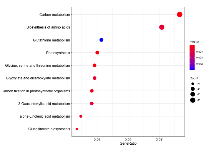
We can then create a dotplot to visualise the KEGG categories significantly enriched.
# create a simple dotplot graph
dotplot(ora_analysis_kegg,
    color = "qvalue",
    showCategory = 10,
    size = "Count")
5.3 KEGG Modules ORA
The KEGG MODULE datase is a series of “manually defined functional units of gene sets”. In particular, pathway modules are functional units of gene sets in metabolic pathways that can give a metabolic-centric view of differentially expressed genes.
The complete list of available modules is available here.
ora_analysis_kegg_modules <- enrichMKEGG(gene = diff_arabidopsis_genes_annotated$entrezgene_id,
                                         universe = all_arabidopsis_genes_annotated$entrezgene_id,
                                         organism = "ath",
                                         keyType = "ncbi-geneid",
                                         minGSSize = 10,           # minimal size of genes annotated by Ontology term for testing.
                                         maxGSSize = 500,          # maximal size of genes annotated for testing
                                         pAdjustMethod = "BH",
                                         qvalueCutoff = 0.05)
Similarly, we can plot this ORA result as a dotplot.
# create a simple dotplot graph
dotplot(ora_analysis_kegg_modules,
    color = "qvalue",
    showCategory = 10,
    size = "Count")
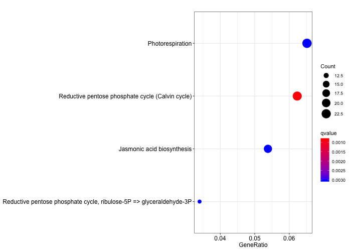
Discussion
Compare the two KEGG plots. Can you identify differences? Which metabolic functions have been grouped together?
6. KEGG ORA analysis for species without a KEGG classification
6.1 kofamscan
If you want to do an overrepresentation analysis on a species that in not in cluded in the KEGG databases, it is posible to manually get ko ids from a protein fasta of the organism you are working on. This can be done using a tool called kofamscan. This tool runs in bash and is available in conda. Not included in this conda tool are the profiles it needs to run. These need to be loaded separately.
create a new conda environment, or run the following in an existing one
$ conda install -c bioconda kofamscan
Download and unzip the required profiles
# download using wget
$ wget ftp://ftp.genome.jp/pub/db/kofam/ko_list.gz
$ wget ftp://ftp.genome.jp/pub/db/kofam/profiles.tar.gz
$ wget ftp://ftp.genome.jp/pub/tools/kofamscan/README.md

# unzip
$ gunzip ko_list.gz
$ tar xf profiles.tar.gz
$ tar xf kofamscan.tar.gz
Run the following on your protein_pep.fasta (in this example I’m using an arabidopsis peptide fasta)
$ exec_annotation --cpu 8 -p profiles -f mapper -k ko_list -o Araport11_genes_ko.txt Araport11_genes.201606.pep.fasta
The file Araport11_genes_ko.txt should have been created. and shoul look something like:
$ less Araport11_genes_ko.txt
AT1G01010.1
AT1G01020.1     K21848
AT1G01020.2     K21848
AT1G01020.3     K21848
AT1G01020.4     K21848
AT1G01020.5     K21848
AT1G01020.6     K21848
AT1G01030.1     K09287
AT1G01030.2     K09287
AT1G01040.1     K11592
AT1G01040.2     K11592
AT1G01050.1     K01507
AT1G01050.2     K01507
AT1G01060.1     K12133
AT1G01060.2     K12133
AT1G01060.3     K12133
AT1G01060.4     K12133
AT1G01060.5     K12133
AT1G01060.6     K12133
AT1G01060.7     K12133
AT1G01060.8     K12133
AT1G01070.1
AT1G01070.2
AT1G01080.1
AT1G01080.2
Araport11_genes_ko.txt
The Araport11_genes_ko.txt file can be downloaded on Zenodo.
6.2 parsing the results
transcriptome <- read.table("Araport11_genes_ko.txt", fill = T, sep = "\t", row.names = NULL, header = F)

differential_genes <- read.table("differential_genes.tsv", sep = "\t", header = T)
Get rid of duplicate transcripts in “universe” through gsub and regex.
transcriptome[,1] <- gsub("\\..*","",transcriptome[,1])
transcriptome <- distinct(transcriptome)
head(transcriptome)
We obtain a list of genes with their corresponding KO term.
         V1     V2
1 AT1G01010
2 AT1G01020 K21848
3 AT1G01030 K09287
4 AT1G01040 K11592
5 AT1G01050 K01507
6 AT1G01060 K12133
6.3 Creating a table ready for hypergeometric p-value calculation
To calculate the p-value associated with each term, we need to calculate:
-
q: the number of genes classified in a given KO term e.g. 10 genes from the list of differentials in K09287. -
m: the total number of genes from the genome classified in this precise KO term e.g. 105 genes from the genome belong to K09287. -
n: the total number of genes from the genome MINUS the number of gene in the given KO term e.g. all genes - the 105 genes from K09287. -
k: the number of genes “drawn” that is the total number of differential genes.
Calculate the total KO term found in the “universe” (i.e. genome). This will be used to calculate the n further.
KITotal <- as.data.frame(table(transcriptome$V2))
KITotal <- KITotal[-1,]
bgTotal <- sum(KITotal[,2])
This gives us a total number of 11,606 KO terms. They are not necessarily unique as some genes map to multiple KO terms just as some genes do not have a KO term assigned to them.
Now to calculate m, the total number of KO terms present in our gene list of interest:
First we filter our “universe” with our gene list, and then calculate the total number of KO terms similarly.
transcriptome_diff_filt <- transcriptome[which(transcriptome$V1 %in% differential_genes$genes),]

KIquery <- as.data.frame(table(transcriptome_diff_filt$V2))
KIquery <- KIquery[-1,]

queryTotal <- sum(KIquery[,2])
This gives us 2439 KO terms.
tableForPhyper <- merge(KIquery, KITotal, by = "Var1")
tableForPhyper$queryTotal <- queryTotal
tableForPhyper$bgTotal <- bgTotal

colnames(tableForPhyper)[1:3] <- c("KOID","queryItem","bgItem")

head(tableForPhyper)
This gives us the following table, ready to calculate the hypergeometric p-value.
KOID     queryItem bgItem queryTotal bgTotal
K00001         3      3       2439   11606
K00002         0      3       2439   11606
K00006         2      2       2439   11606
K00008         1      1       2439   11606
K00012         1      4       2439   11606
K00013         0      1       2439   11606
6.4 Calculate the hypergeometric p-value
Run hypergeometric test using the phyper() function and to perform multiple test correction at the same time.
res <- tableForPhyper %>%
  rowwise() %>%
  mutate(p_val = phyper(q = queryItem, m = bgItem, n = bgTotal-queryTotal, k = queryTotal)) %>%
  mutate(p_adj = p.adjust(p = p_val, method = "fdr"))
head(res)
  KOID   queryItem bgItem queryTotal bgTotal p_val p_adj
   <fct>      <int>  <int>      <int>   <int> <dbl> <dbl>
 1 K00001         3      3       2439   11606 1     1
 2 K00002         0      3       2439   11606 0.395 0.996
 3 K00006         2      2       2439   11606 1     1
 4 K00008         1      1       2439   11606 1     1
 5 K00012         1      4       2439   11606 0.711 0.996
 6 K00013         0      1       2439   11606 0.734 0.996
 7 K00014         1      1       2439   11606 1     1
 8 K00016         0      1       2439   11606 0.734 0.996
 9 K00020         1      7       2439   11606 0.406 0.996
10 K00021         1      2       2439   11606 0.929 1
7. Gene Set Enrichment Analysis (GSEA) with ClusterProfiler
The Gene Set Enrichment Analysis (GSEA) is another way to investigate functional enrichment of genes and pathways using the Gene Ontology classification. Please refer to the following section in Prof. Guangchuang Yu book for a clear explanation of GSEA and how to implement it with clusterProfiler.
The above sections can of course be run on species other than arabidopsis. In most cases it is sufficient to change the initial biomartr query from section 3.4 to the species you are investigating.
For example with tomato:
biomartr::organismBM(organism = "solanum lycopersicum")
tomato_attributes =
biomartr::organismAttributes("solanum lycopersicum") %>%
filter(dataset == "slycopersicum_eg_gene")
tomato_attributes
Of course with these changes, you should also change the variables associated with the organism. In some species, however, this method leads to quite a reduction in the number of genes that get translated to GO terms or KEGG IDs.
8. Going further
8.1 Useful links
8.2. References
- The Cluster Profiler companion book, a great place to start
- Zhou et al. (2019). Metascape provides a biologist-oriented resource for the analysis of systems-level datasets. Nat Commun 10, 1523 (2019). link
- Yates et al. (2020) Ensembl 2020, Nucleic Acids Research, Volume 48, Issue D1, 08 January 2020, Pages D682–D688, Link
- Tian et al. (2017) agriGO v2.0: a GO analysis toolkit for the agricultural community. Nucleic Acids Research, Volume 45, Issue W1, Pages W122–W129.Link
- Drost et al. (2017) Biomartr: genomic data retrieval with R. Bioinformatics 33(8): 1216-1217. doi:10.1093/bioinformatics/btw821.
Key Points